Clatter from the Byte Kitchen

This is part 1.1 of a number of blog posts on parallel stream compaction

In part 1 we saw that the parallel stream compaction Cuda software by Billeter et al. is faster than the software by Orange Owls , which in turn is faster than the software by Spataro. Commenter Qubey then asked if this relative order is preserved under migration to other graphics cards, notably to graphics cards with newer generations GPU’s. This is an important question because it addresses the validity of a choice for a particular algorithm (and its implementation) for future hardware. This validity depends largely on adherence to an architectural model in successive hardware generations and the software runtime environment.

We set out to experiment. All three implementations will be run with structured data for streams of size 2^10 up to and including 2^26. Structured data is of the form 1, 0, 3, 0, 5, 0, 7, 0, … Values are limited to [0, 2^16 – 1]. We have seen in part 1 that the algorithms are not sensitive to structure in the input data. This was also found in the extensive experiments reported on here (although we will not discuss it further). The implementations of Orange Owls and Spataro will be run for 32, 64, …, 1024 threads per block. The thread layout of the Billeter et al. implementation is fixed. We ran this software on various graphics cards: a GeForce GTX 660, 690, 960 and 1080. Time performance measurements are averaged over 1,000 calls of the kernel.

The questions we would like to see answered are:

1. Is the relative ordering in time performance of the implementations preserved over the different graphics cards?
2. Is the time performance relation between the fastest implementation and the runner up implementation constant over the different graphics cards? Can we say that implementation X Is Y times faster than implementation Z?

Relative order

The first question can best be answered by presenting time performance graphs of the cards involved.

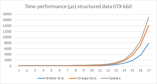
Explanation of the numbers on the x-axis: x=1 means the input length is 2^10, x=2: input size is 2^11, … x=17: input size = 2^26. This holds for all graphs below.

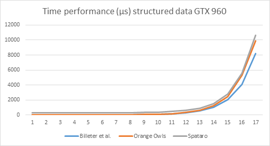
It is obvious from the graphs that relative ordering of performance is preserved over the cards.

Note by the way the enormous increase in time performance. The GTX 660 takes almost 8ms to process the largest stream (2^26 elements) using the Billeter et al. algorithm, whereas the GTX 1080 needs only 3ms.

Magnitude

The data from part 1 suggests that there is a multiplicative relation between the fastest algorithm: Billeter et al., and the runner up: Orange Owls. The data from the current test set support this suggestion, as the following graphs illustrate.

The graphs below show (i) the Orange Owls time performance measurements divided by the Billeter et al. measurements; (ii) Spataro divided by Billeter et al.; and (iii) Spataro divided by Orange Owls.

We see that the division of the Orange Owls data divided by the Billeter et al. data, reasonably approximates a straight line, indicating an approximately constant factor on all cards. This will allow us to say something like “The implementation by Billeter et al. is X times faster than the implementation by Orange Owls.” The other two relations are clearly not of this nature.

We see that there is indeed a multiplicative relation between the Billeter et al. and Orange Owls time performance data. So what is the magnitude of these relations for the different cards, and are they more or less the same? Take a look at the table below.

As you can see, mean and standard deviation are similar over the cards, with the exception of the GTX 960. I’ll get to that. Based on these results, I’m inclined to say that Billeter et al. stream compaction is about 1.5 times as fast as Orange Owls stream compaction.

On the other hand, the magnitude of the multiplicative relation seems to be about 1.6, with the notable exception of the GTX 960. We note that the theoretical memory bus bandwidth of the GTX 960 is (only) 112 GB/s for the reference card and 120 GB/s for OEM cards (Wikipedia), whereas the bandwidth of the GTX 660 is 144 GB/s, and for the 690: 192 GB/s (per GPU).

The time performance comparison chart for all cards on structured data, Billeter et al. implementation looks like this:

Which shows that the GTX 960 is relatively less suited for stream compaction compared to the other cards.

Wrapping up

In part 1: Introduction, based on one graphics card and a single input stream size, Billeter et al. came out twice as fast as Orange Owls. This finding has now been developed into a factor 1.5 by the introduction of a broad spectrum of cards and a far broader scope of input streams. We have seen that Billeter et al.’s implementation of stream compaction is the fastest, for a substantial number of input stream lengths and over a number of graphics cards generations.

Next

Next we will start digging into the inner workings of the algorithms, as promised in the introduction.

Thanks

I would like to express my gratitude to Qubey for his sharp questions and for his willingness to conduct experiments on the GTX 660, 960 and 1080 cards.

What is Stream Compaction

Stream compaction is simply copying only the nonempty (valid) entries from an input array to a contiguous output array. There is, of course, the option to not preserve the order of the input, but we will skip that one.

In C++ the definition is simple. Given a sparse std::vector<T> v_in, and an equal sized, zero std::vector<T> v_out:

auto j = 0u;
for (const auto& e : v_in)
{
	if (e) v_out[j++] = e;
}

where T is the value type of both v_in and v_out.

If you apply this sequential algorithm to real time graphics tasks, you will find that it is too slow (we will get to the numbers below).

On the other hand, stream compaction is a very important algorithm in general purpose GPU (GPGPU) computing, and/or data parallel algorithms. Why? Typically, GPGPU algorithms have fixed output addresses assigned to each of the many parallel threads (I will not explain data parallel algorithms here, please do an internet search if new to this subject).

Not all threads produce (valid) output, giving rise to sparse output arrays. These sparse output arrays constitute poor quality input arrays for subsequent parallel processing steps: it makes threads process void input. Understandably, the deterioration may increase with an increasing number of processing steps. Hence the need for stream compaction.

World Champion Parallel Stream Compaction

Some time ago I needed a GPU stream compaction algorithm. Of course, initially I was unaware of this term, just looking for a way to remove the empty entries from a large Direct3D buffer. Internet research taught that there are a few fast implementations: by Hughes et al. [3], Spataro [2], and Billeter et al.[1]. And let’s not forget the Cuda Thrust library which contains a copy_if function (Cuda release 8). Software implementations can be downloaded from [6], [5], [4], and [7] respectively.

I’ve benchmarked the implementations on my Asus Geforce GTX 690, also including an implementation of Spataro’s algorithm by Orange Owls [8]. Two input vectors have been used:

1. A structured vector [1, 0, 3, 0, 5, 0, 7, … ].
2. A vector of pseudo random unsigned shorts, selected by rand(), with an approximate probability of 50% to be zero (decided using rand() also).

Both vectors have size 2^24 (almost 16.8 million).

The table below displays the results of running standard Visual Studio 2015 release builds without debugging. Measurements are averaged over 1,000 executions of the involved kernels. Measuring code directly surrounds the kernel calls. Outcomes have been checked for correctness by comparison with the outcome of the sequential algorithm above. All algorithms produce correct results.

So what do we see?

We see that the CPU code produces strongly varying results for the two input vectors. Parallel implementations do not suffer from this variance (or do not benefit from structure that is inherent in the data!).

The algorithm by Billeter et al.’s is at least twice as fast as the other algorithms. It is a step ahead of Spataro, Orange Owls, and Thrust.

Obviously, there is something wrong with Hughes et al.’s algorithm, or its implementation. According to the article [3], it should be faster than, or on par with Billeter et al.’s. Obviously, it isn’t. Inspection using the NVidia Visual Profiler shows that the threads are mainly (over 90%) ‘Inactive’, which explains its lack of performance.

Having read the articles referred to above, I decided to see if I myself could become world champion parallel stream compaction, by writing a new algorithm based on some ideas not found in the articles. So, could I be the new world champion? No. I got results in between Orange Owl’s and Spataro’s, but could not get any faster.

So, the software by Markus Billeter, Ola Olsson, and Ulf Assarsson is the fastest parallel stream compaction algorithm in the world, they are world champion stream compaction, and we have to first learn why exactly, before we can surpass it, if at all. The question that then is:

“What makes Billeter, Olsson, and Assarsson’s parallel stream compaction Cuda program at least 2x as fast as its competitors?

Next

The implementation of Billeter et al.’s algorithm is an optimized library. Optimized also with respect to maintenance: no duplicate code, which makes it fairly cryptic, thus hard to decipher its operational details. Next up is a general description of their program, and its main parameters. The algorithm has three main steps which will be discussed in subsequent posts. Along the way I hope to disclose why their code is at least twice as fast as the other algorithm implementations.

References

[1] Billeter M, Olsson O, Assarsson U: Efficient Stream Compaction on Wide SIMD Many-Core Architectures. In Proceedings of the Conference on High Performance Graphics Vol. 2009 (2009), p. 159-166.
New Orleans, Louisiana — August 01 – 03, 2009. ACM New York, NY, USA. (http://citeseerx.ist.psu.edu/viewdoc/download;jsessionid=4FE2F7D1EBA4C616804F53FEF5A95DE2?doi=10.1.1.152.6594&rep=rep1&type=pdf ).

[2] Spataro Davide: Stream Compaction on GPU – Efficient implementation – CUDA (Blog 23-05-2015: http://www.davidespataro.it/cuda-stream-compaction-efficient-implementation/ ).

[3] Hughes D.M. Lim I.S. Jones M.W. Knoll A. Spencer B.: InK-Compact: In-Kernel Stream Compaction and Its Application to
Multi-Kernel Data Visualization on General-Purpose GPUs. In: Computer Graphics Forum, Volume 32 Issue 6 September 2013 Pages 178 – 188. (https://github.com/tpn/pdfs/blob/master/InK-Compact-%20In-Kernel%20Stream%20Compaction%20and%20Its%20Application%20to%20Multi-Kernel%20Data%20Visualization%20on%20General-Purpose%20GPUs%20-%202013.pdf ).

[4] Source code Billeter, Olsson, and Assarsson: https://newq.net/archived/www.cse.chalmers.se/pub/pp/index.html .

[5] Source code Spataro: https://github.com/knotman90/cuStreamComp

[6] Source code Hughes, Lim, Jones, Knoll, and Spencer: https://sourceforge.net/projects/inkc/

[7] Cuda 8 (September 2016 release, includes Thrust): https://developer.nvidia.com/cuda-toolkit .

[8] Orange Owls Solutions implementation of Spataro’s: https://github.com/OrangeOwlSolutions/streamCompaction

For those interested: I have prepared three programs that experiment with the Cuda stream compaction implementions of Billeter et al., Spataro and Orange Owls. You can request download links (executables and sources) by creating a comment.