Clatter from the Byte Kitchen

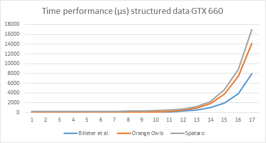
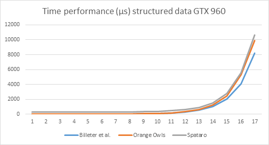
This is nr. 5 in a collection of blog posts on Parallel Stream Compaction. And this will be the final episode. In previous posts we saw that the implementation by Billeter, Olsson, and Assarsson is faster than implementations by Orange Owls and Spataro; a multiplicative relation holds for processing times, even over different graphics cards. We saw that the essential differences between the fastest algorithm, by Billeter et al., and the others, are that the former uses sequences, a very small data structure for metadata, and vectorized IO, and that the latter programs do not.

In the previous post we saw that in particular vectorized IO makes the performance difference between the slower and the faster programs.

This post discusses a somewhat modernized and optimized library for stream compaction, put together from code of different sources and my own efforts.

Modern constructs for Billeter et al.

The stream compaction code by Billeter et al. predates the Cuda __shfl_x constructs which allows for very concise scan and reduce functions. Thus, their program can be rearticulated in significantly shorter code. Taking their program as a starting point, along with code fragments from other sources, I have constructed another stream compaction program. The core algorithm takes about 150 lines of spacious code.

A disclamer is required here. I do not (yet) own the lastest Cuda capable hardware. So, there are modern constructs that are not applied, which would simplify the code and enhance its performance further. In particular, one might think of dynamic parallellism which would allow for a stream compaction algorithm without the construction and use of any metadata at all. On the other hand, this same modern hardware dwarfs the performance of my GeForce GTX 690, which would render further optimization pretty senseless.

Optimization

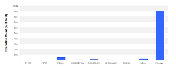
We have learned a number of lessons about optimal implementations of the various phases of stream compaction in the previous episodes of this series. This concerns using sequences, vectorized IO, threading configuration, and also the use of warp level primitives that eliminate some uses of shared memory in this program (namely to support inter thread, intra warp data exchange).

Applying these lessons leads to a stream compaction library that is even faster than Billeter et al.’s.

One somewhat brutal optimization is to eliminate the ability to process the exact size of the input stream. The library I pieced together from various sources requires an input stream which length is a multiple of 65.536 (2^16 = 64K). This seems a large number, but all is relative. First of all, if you have a small stream, compaction is just as well done using CPU code. If, on the other hand, you have a large input stream, even a number like 65.536 is only a small fraction of this large stream. For instance 65.536 x 19 = 1.245.184: a moderately large stream. Now, 64K is 5.3% of 1.245.184. If we take 65.536 x 20 = 1.310.720 instead, we have an overhead of 5.3% – 5% = 0.3%. Note that there may be a performance advantage in taking the larger size, see below.

How does this multiple of 64K come about? If you have a large stream, we will first divide it up into 512 sequences that are processed as concurrently as possible. Each sequence is read using uint4 vectorized IO, which divides its length by 4. The resulting chunk should be a multiple of the warp size (so it can be processed concurrently per warp). Then we have that 512 x 4 x 32 * i = 65.536 * i (i the multiple of 32). I found that the advantage of rounding up to the next multiple of 64K is pretty robust for very large streams.

The requirement that the input length is a 64K multiple is a consequence of the configuration of the algorithmic parameters, and a corresponding selection of code from the demo code into the library. The code can be customized to fit specific applications by changing the number of sequences and/or changing the level of vectorized IO. E.g. if you set the number of sequences to 1, and restrict to scalar IO, the requirement reduces to the input length being a multiple of the warp size (32 for now).

Comparison to Billeter et al.

So let’s go to the numbers. How do performances compare, overall, and for different phases? All measurements are for rand() data with a rand() % 2 choice for a nonzero (== valid) value.

N = 2^24.

So, the new library is a bit faster in all phases.

Other input sizes

Now let’s explore the performance of the library with other input sizes.

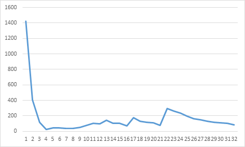
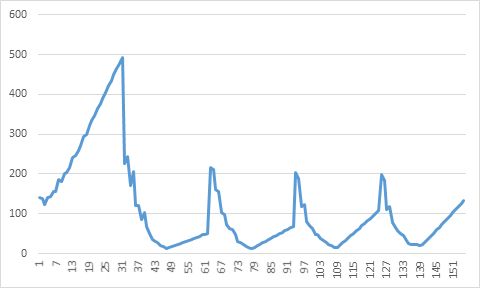
If we let the library process input stream of length 65536 * i with i = 1, …, 256 (65536 * 256 == 2^24), we may get the following graph.

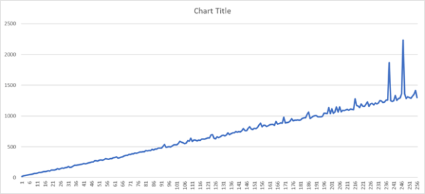
This is a kind of a surprise. I ran the program several times, and the results have a somewhat statistical character, but one or two peaks at the end of the x-axis are always there.

What do we see?

• For smaller values of the size we see a pretty regular development, but for some input lengths, processing times are shorter than for somewhat smaller lengths.
• For larger values, extreme differences in processing times between subsequent input sizes are possible.

So, it pays to see if a somewhat longer input length yields a shorter processing time. In case of rounding to the nearest multiple of 64K one can of course investigate whether adaptation of the algorithmic parameters and code selection provides better results.

Demo code

Below, two links to code are inserted. One link is to a demo program. This program has an IO variant for each phase. The other link is to the library, as discussed above. All code is currently for unsigned int.

ParallelStreamCompaction5

Stream_compaction_lib

This is nr. 4 in a collection of blog posts on Parallel Stream Compaction. In previous posts we saw that the implementation by Billeter, Olsson, and Assarsson is faster than implementations by Orange Owls and Spataro; a multiplicative relation holds, even over different graphics cards. We saw that the essential differences between the fastest algorithm, by Billeter et al., and the others, are that the former uses sequences and a very small data structure for metadata, and the latter programs do not.

In the previous post we saw that the introduction of sequences in itself does not provide a performance advantage. The question we address here is: Can the sheer volume of the metadata account for the performance differences?

The size of the meta data structure

The element counts of the metadata structures corresponding to best time performance on a stream of 2^24 elements are:

• 512 unsigned ints in Billeter, Olsson, and Assarsson’s algorithm.
• 16,384 ints in Spataro’s algorithm.
• 16,384 ints in Orange Owls’ implementation of Spataro

Billeter et al. have a metadata structure of 512 elements (of which they use 480 elements). The size is set at compile time and is part of a configuration the authors deem optimal. If you do not change the code, the size fixed.

The size of the metadata structure in Spataro’s and Orange Owls’ code equals the number of blocks, hence it varies with the threading configuration. In the first post in this series we determined the best time performance for a stream of 2^24 ints of both programs. The nr of elements in the metadata structures corresponding with the best performance was 16,384 in both cases.

The large difference in size is a consequence of design: Spataro’s and Orange Owls’ algorithms collect metadata per block of threads. Billeter et al.’s: code collect metadata per sequence.

Parameter search

To find out if there are significant differences, I did a parameter search for optimal numbers of threads per block and the number of thread blocks for two approaches:

1. With sequences; the number of elements in the metadata array equals 512.
2. Without sequences; the number of elements in the metadata array equals the number of blocks.

The test code that made the comparisons again uses a stream of 2^24 unsigned ints, selected in a rand() way. The fraction of valid elements is about one half, again decided by rand(). Both approaches were tested with scalars, pairs and quads.

Sequence wise algorithm

The small volume metadata code uses a warp size stride sequence algorithm. Starting from 128 threads per block with 128 blocks (a generalization of Billeter et al.’s threading configuration), I varied the numbers but held the product constant: 128 x 128 = 64 x 256 = 32 x 512, and vice versa, so a 512 element metadata structure suffices.

The main code for scalars look like this:

// Nvidia example code
template <typename T>
__inline__ __device__ T warpReduceSum(T val)
{
	for (auto offset = warpSize / 2; offset > 0; offset /= 2)
	{
		// Accumulate values over the warp
		val += __shfl_down(val, offset);
	}

	return val;
}

__global__ void device_prefix_kernel2(const unsigned int* d_in, unsigned int* d_out,
const unsigned int seq_size)
{
	// Global thread index
	const auto idx = blockIdx.x * blockDim.x + threadIdx.x;

	// index within warp
	const auto lane = threadIdx.x % WARP_SIZE;
	// global index for warp, sequence
	const auto sidx = idx / WARP_SIZE;
	// Start of the sequence in the input array
	const auto seq_begin = seq_size * sidx;
	// End of the sequence
	const auto seq_end = seq_begin + seq_size;

	// Work the sequence in a warp
	auto sum = 0u;
	for (auto i = seq_begin + lane; i < seq_end; i += WARP_SIZE) { sum += d_in[i] > 0;
	}

	// Accumulate the warp local sums
	const auto cnt = warpReduceSum(sum);

	// Write output
	if (lane == 0)
		d_out[sidx] = cnt;
}

Block wise algorithm

The large volume metadata main code for scalars looks this:

// After Spataro
__global__ void device_count_kernel1(unsigned int* d_in, unsigned int* d_out)
{
	// Determine global thread index
	const auto idx = blockIdx.x * blockDim.x + threadIdx.x;

	// Read input value
	const auto val = d_in[idx];
	// Count all positive values 
	const auto cnt = __syncthreads_count(val > 0);
	// Write the output
	if (threadIdx.x == 0)
		d_out[blockIdx.x] = cnt;
}

A link to the complete demo code can be found at the bottom.

Time performance results

The table below shows the performance for both alternatives; for thread counts that seem to fit the algorithms best.

	Block Wise (µs)		Sequence Wise (µs)
Threads	512 (16,384 blocks)		64 (256 blocks)
Scalar	771.0		502.1
uint2	509.6		445.1
uint4	448.2		445.4

We see that the block wise algorithm can take great advantage of vectorized reads. For uint4 the algorithm is just as fast as the sequence wise algorithm. The latter can take only limited advantage of vectorized reads, but is in itself blazingly fast.

Lesson Learned

Compare these results to the table in part 2 of this series. In that table Billeter et al. have 455.5 µs for the count phase. They use vectorized reads with pairs. Notice how similar the time measurements in both tables are for this IO configuration. Spataro and Orange Owls however, use scalar based IO, which is much slower. This then is the explanation why the code by Spataro and Orange Owls is slower than that by Billetter et al.: The formers do not use vectorized IO! It also explains why the difference in time performance is a factor, i.e. has a multiplicative character: Billeter et al. read and write twice as much data in a single action.

So, the code by Spataro and Orange Owls could have been just as fast as the code by Billeter et al., if they just had used vectorized IO. It is neither the use of sequences, nor the size of the metadata structure.

This is an important lesson: It is knowledge of the language and platform facilities that makes a program the fastest one, or a slower one.

Demo Code

The complete demo code for this blog post can be downloaded from here.

Next

Next up: Now that it is clear that all three implementations of parallel stream compaction that have been explored in this blog post series could have had about equal performance, I would like to combine the software I wrote or adapted from the sources investigated, into a short and fast program for parallel stream compaction.

This is nr. 3 of some blog posts on Parallel Stream Compaction. In previous posts we saw that the implementation by Billeter et al. is a factor faster than implementations by Orange Owls and Spataro, and that a multiplicative relation exists, even when using different graphics cards. We wondered if the essential difference between the implementations is that the former uses loops that process the input in subsequences, and the latters do not.

In this post we will examine loops and sequences in a Cuda copy program, a simpler context than stream compaction. The program takes a long array and returns a copy. Simple as that. The question here is if the use of loops can account for the difference in performance mentioned above, and if so, can we say something about optimal parameter configurations.

This investigation compares loops and subsequences set up according to Billeter et al. to not using loops at all, “grid stride loops” as advocated by Nvidia [1], and warp stride loops which is a generalization of the way Billeter et al. organize loops. For the latter three algorithms we will do a parameter search to (by and large) optimize parameter settings. Recall that the former algorithm has fixed parameters for the number of threads per thread-block and the number of blocks

A link to sample code can be found at the bottom of this post. (not yet, but on its way!)

No loops, Grid stride loops, Billeter et al. loops, and Warp stride loops

The task will be to copy an array of 2^24 elements. The elements are chosen using c++ rand();

No loops

If we do not use loops or sequences we can copy the array with a function like the one below. It is a template, so we can easily experiment with different types of arguments.

template 
__global__ void device_copy_kernel1(T* d_in, T* d_out)
{
	// Determine global index into the arrays
	int idx = blockIdx.x * blockDim.x + threadIdx.x;

	// Copy the element
	d_out[idx] = d_in[idx];
}

I used arrays of unsigned int in the experiments described here.

Grid stride loops

When using grid stride loops, the step size equals the entire grid of threads. The size of a grid is

number-of-threads-per-block x number-of-blocks

i.e., the entire number of threads used by the program. We can choose the total number of threads freely, but if we also choose wisely, it is a divisor of the array size, and we choose the block size to be a multiple of the warp size: 32 for current hardware. The maximum block size is 1024.

A simple function to copy an array using grid stride loops is the following.

template
__global__ void device_copy_kernel2(T* d_in, T* d_out)
{
	int idx = blockIdx.x * blockDim.x + threadIdx.x;

	for (int i = idx; i < ARRAY_SIZE; i += blockDim.x * gridDim.x)
	{
		d_out[i] = d_in[i];
	}
}

Billeter et al. loops, Warp stride loops

Billeter et al. have set the number of threads per block to 128, and the number of blocks to 120. They also have a complex way to cut up an array into subarrays. Well, for now I will cut up the array in equal sized chunks. If performance results are close, there is always the option to go into more complexity.

A distinguishing feature of the Billeter et al. loop is that is has a warp size stride. We might find it interesting to explore this feature further, so let’s use the following function.

template
__global__ void device_copy_kernel3(const T* d_in, T* d_out, const unsigned int seq_size)
{
	const auto idx = blockIdx.x * blockDim.x + threadIdx.x;

	// index within warp, the name lane refers to the hardware implementation
	const auto lane = threadIdx.x % WARP_SIZE;
	// global index for warp, sequence
	const auto sidx = idx / WARP_SIZE;

	// set sequence begin and end
	const auto seq_begin = seq_size * sidx;
	const auto seq_end = seq_begin + seq_size;

	// copy the sequence
	for (auto i = seq_begin + lane; i < seq_end; i += WARP_SIZE)
	{
		d_out[i] = d_in[i];
	}
}

the seq_size parameter is defined as:

const unsigned int seq_size = ARRAY_SIZE / warp_cnt;

where warp_cnt is:

const unsigned int warp_cnt = (threads * blocks) / WARP_SIZE; // WARP_SIZE = 32

Benchmarks

Time measurements are averaged over 1000 calls of the kernel; Visual Studio release builds that are run without debugging, on an Asus Geforce GTX 690.

No loops

For the No loops case we cases we let the number of threads per block run from 32 – 1024 in steps of 32, the number of blocks is just ARRAY-SIZE / number-of-threads-per-block.

This gives us the following graph (I have subtracted 850 µs from each time measurement, in order to enhance the differences; all time measurements are larger than 850 µs).

There is a global minimum around the fourth measurement, i.e. in this experiment, the fourth measurement provides the best time performance.

Grid stride loops

The Grid stride loop case has a huge number of possible parameter values, so we do a somewhat coarse search. The set of numbers of threads per block is {64, 128, 256, 512, 1024}. The parameter space for the number of blocks is divided into 32 values (where we disregard the case for zero blocks).

This gives us the following graph (I have again subtracted 850 µs from each time measurement).

The are several, let’s say, regional minima: the 47th, 78th, 109th, and 139th measurement.

Interestingly, this is a very regular series. The last measurement is just 1 step before the step with 8192 blocks (2 x 8192 = 16384).

Warp stride loops, Billeter et al. loops

Nvidia hardware executes a warp of threads in parallel on a single multiprocessor. So it makes sense to set up sequences that are processed by a single warp of threads. Such sequences are processed by warp stride loops. The number of warps then determines the number of sequences, hence their size. NVidia warns not to write programs that critically depend on the size of a warp. So, production software that uses the warp size as a parameter should always query the hardware at runtime to get the actual warp size (for the overseeable past and future expect it to be either 16, 32, or 64).

Billeter et al. have a warp stride loop with 120 blocks of 128 threads. I have measured the time performance and registered it in the table in the Summary section.

The time performance is not ultimately impressive: 1804.7 µs; the slowest option in the pack .

In order to see if the warp stride loop variant has any merits, I performed a parameter search, similar to the grid stride loop case. Note that the array length, the warp size, the number of threads per block, and the number of blocks together completely determine the size and number of sequences.

This resulted in the following graph (each measurement got again 850 subtracted).

The 47^th measurement has the shortest time: 863.7 µs.

Summary

The best time performance and bandwidth results are in the table below.

	Time (µs)	Bandwidth (GB/s)	Threads	Blocks	Sequence size
No Sequences	870.9	154.1	128	131,072	–
Grid Stride Loops	861.8	155.7	800	1,024	array size
Billeter et al. Sequences	1,804.7	74.4	128	120	32,768
Warp Stride Loops	863.7	155.4	128	65,536	64

Time is in microseconds, so all results are about equal, except the Billeter et al. case which is significantly slower.

At this point we see no (dis)advantage of using sequences!

Vectorized Memory Access

Another question is if any of these alternatives can can benefit from using vectorized memory access [2]. The hardware can execute memory access operations on scalars, but also on small vectors of 2 components (pairs) or 4 components (quads). To see what the effects of vectorized memory access are, I adapted the software accordingly. Note that if the program processes vectors of e.g. 4 components, it need only 1/4th of the reads and writes of the scalar case.

Vectorized memory access with pairs

The test program proceeds just as described above. The table below summarizes the results obtained.

	Time (µs)	Bandwidth (GB/s)	Threads	Blocks	Sequence size
No Sequences	857.9	156.5	704	11,915	–
Grid Stride Loops	859.7	156.1	1,024	8,192	array size
Billeter et al. Sequences	1,434.6	93.6	128	120	17,464
Warp Stride Loops	820.9	163.5	256	38,912	26

It turns out that warp stride loops benefit most from vectorized memory access with pairs. This includes Billeter et al. sequences.

Vectorized memory access with quads

The table below summarizes the results obtained.

	Time (µs)	Bandwidth (GB/s)	Threads	Blocks	Sequence size
No Sequences	862.3	155.7	1,024	4,096	–
Grid Stride Loops	862.4	155.6	64	65536	array size
Billeter et al. Sequences	1,335.7	100.5	128	120	8738
Warp Stride Loops	831.7	161.4	256	38,912	26

So, it seems that vectorized memory access with quads, as opposed to pairs, is beneficial for Billeter et al. sequences, but not for the other options.

Conclusions

We conclude that warp stride loops offer the best performance. Better than using no loops, to be sure, if combined with vectorized memory access for pairs (not quads).

We have seen that the performance graphs of the various options show many local minima. So, it pays to do a search for the parameters that maximize performance.

Then, of course, there is the question whether sequences is what makes Billeter et al stream compaction the world champion. The answer is: Definitely not!

Addendum / Correction

<11-06-2018> Cleaning up the demo software I noticed that the Billeter et al. case had the code for setting up the sequences included in the time measurement section, whereas setting up sequences is a compile time activity in the original program by Billeter et al. So, when this is corrected, processing times become significantly better, 1125.3 µs (119.3 GB/s) for the scalar case, 1005.6 µs (133.5 GB/s) for pairs, and 1023.8 µs (131.1 GB/s) for quads respectively. Note however, that the general conclusions do not change.

Next

If the use of sequences does not set stream compaction according to Billeter et al. apart from the rest, then what does? Is it the difference in size the meta data volume?

References

[1] https://devblogs.nvidia.com/cuda-pro-tip-write-flexible-kernels-grid-stride-loops/

[2] https://devblogs.nvidia.com/cuda-pro-tip-increase-performance-with-vectorized-memory-access/ .

Demo code

You can download demo code from here

This is number 2 of some blog posts on Parallel Stream Compaction. In part 1 we saw a small number of fast implementations compared. The implementation by Billeter Olsson and Assarsson came up as the fastest. In a digression of different graphics cards we saw that the order in performance holds over different cards, over different generations. Now we want to know why the implementation by Billeter et al. is so distinctively faster than the other two.

In this part we measure time performance of the individual steps that comprise the algorithms, and discuss the results before we dig in deeper in further episodes. The code we use here is the code discussed in part 1.1: the digression comparing various graphics cards.

Measuring time performance of the three processing steps

All algorithms discussed in part 1 have three sequential steps, where each step is a Cuda kernel:

1. Count the number of valid entries. The Count step.
2. Determine the global offsets in the output for the entries. The Prefix step.
3. Compact the valid entries into the output using the offsets. This is the Move step.

So, the first two steps provide metadata, and the third step uses the metadata to compact the stream.

The time performance of the separate steps may show us bottlenecks in the implementations.

We benchmark the individual steps with structured data (see part 1) on a GeForce GTX 690. We use the software from part 1.1, but restrict the size to 2^24. In the case of the Orange Owls and Spataro implementations, we restrict the threading configuration to 1024 threads per thread-block. This latter choice came out as the fastest thread configuration for the specified input length.

Measuring processing time is as follows. The individual steps are measured indirectly: first we measure step 1, then we measure step 1 and 2, and subtract step 1, etc. Time is measured in microseconds (µs = 10^-6 seconds). Measurement times are averages over 1,000 invocations.

We then see the following results.

	Count (µs)	Prefix (µs)	Move (µs)	Total (µs)
Billeter et al.	455.5	7.3	820.0	1282.8
Orange Owls	893.6	47.2	1665.8	2606.6
Spataro	946.6	86.6	2107.9	3141.1

Let’s discuss this a bit.

The Prefix Step

The prefix step by Billeter et al. is much faster than the prefix step in the other two implementations. Curiously, both Orange Owls and Spataro employ the thrust::exclusive_scan function. This function is part of the Thrust library that is packed and distributed with the Cuda SDK(!). Ok, we already know from part 1 that Thrust is not the ultimate in performant GPU software, but the difference with Billeter et al. is really too large.

We will discuss Billeter et al.’s prefix step in a later episode in detail.

The Count and Move steps: loops

A major difference between the implementation by Billeter et al. and the other two is that the former employs loops.

Loops, as in sequential processing? In massively parallel software? And then having a performance advantage??? Yes!

Here is a count function from the source code by Billeter at al. that loops through an array.

template< class Pred > static _CHAG_PP_DEV SizeType count(
    const T* aStart, const T* aEnd, const Pred& aPred, volatile SizeType* aSmReduce)
{
    SizeType partialCountA = 0u, partialCountB = 0u;
    for(const _Tp* elem = _Tpp(aStart) + _Env::lane(); elem < _Tpp(aEnd);
        elem += _Env::SIMD)
    {
        _Tp e = *elem;
		
        if( aPred( e.x ) )
	    ++partialCountA;
        if( aPred( e.y ) )
	    ++partialCountB;
    }
	
    SizeType sum = partialCountA + partialCountB;

    return _Unit::reduce( sum, op::Add<SizeType>(), aSmReduce );
}

Notice the for loop, it defines how each thread of a warp iterates through the input from aStart (plus the offset for the thread) up to aEnd, with increments of the warp size (so threads do not get in each other’s way).

Here is the count function from Orange Owls. No loops at all.

template <typename T, typename Predicate>
__global__ void computePredicateTruePerBlock(const T * __restrict__ d_input,
    const int N, int * __restrict__ d_BlockCounts, Predicate predicate)
{
    int tid = threadIdx.x + blockIdx.x*blockDim.x;

    if (tid < N)
    {

        int pred = predicate(d_input[tid]);
        int BC = __syncthreads_count(pred);

        if (threadIdx.x == 0) { d_BlockCounts[blockIdx.x] = BC; }
    }
}

What does this code do? First it determines a global index for the current thread (tid), then, if the index denotes a location in the input, it determines if a predicate holds for the designated input, by setting a variable to 1 if it does, and to 0 if it doesn’t. It then sums all the outcomes in a warp, and stores the result.

Default threading configuration in Billeter et al.

The threading configuration in Billeter et al. depends on compile time parameters. The default configuration for step 1 (Count) and step 3 (Move) is that processing takes 120 blocks of 128 threads each. This is surprisingly low! Can we even speak of data parallelism? The 128 threads of a block have been subdivided in 4 warps of 32 threads: dim3(32, 4, 1). In contrast: the Prefix step uses 480 threads in 1 block.

The total number of threads (128 x 120) is far less than the size of the input stream. So, the algorithm employs sequences: ordered, contiguous, nonoverlapping subarrays; an order preserving concatenation of the sequences equals the input stream.

Number of sequences

The parallelism in GPU computing is per warp. So, the number of sequences in this algorithm is the total number of warps, which is the number of warps per thread-block x the number of blocks (4 x 120 = 480). The Count step counts the valid entries of the input per sequence and outputs an array of the counts, just as the Move step moves the valid entries to the output per sequence. The Prefix step takes as input the output of the Count step which has length 480. Since the Prefix step has 480 threads, there are no sequences in the Prefix step.

Note that the small numbers of thread-blocks and threads per block result in small data structures for the counts-of-valid-elements-per-sequence, and the global-offsets-per-sequence. I think that having small metadata data structures is a performance factor in itself.

Size of the sequences

Billeter et al. compute the size of the sequences using a rather complicated recipe:

1. Determine the size of a data block a warp processes in one call. For instance, if we use the uint2 short vector type (of 2 unsigned ints), this is the warp size x the number of unsigned ints in a uint2. Hence, 32 x 2 = 64.

1. Compute the basic sequence size as the stream size divided by the data block size, and then divided by the number of sequences. Note that these divisions are integer divisions. In our case: 2^24 / 64 = 262,144, then 262,144 / 480 = 546 with a remainder of 64.
2. Add the remainder R to the size of the first R sequences.

So, in our input of size 2^24, the first 64 sequences have size 35008, and the other 480 – 64 = 416 sequences have size 34944.

The code is flexible and can work with very arbitrary length input streams. If the length of an input array is not a multiple of the warp size, the code calculates a range of auxiliary input elements and processes these separately. I will argue against this solution elsewhere, for now we can ignore this facility since the (large) size we use for experiments is a power of 2 – hence a multiple of 32.

Next

If we want to conclude that the performance difference between the implementation of Billeter et al. on the one hand, and Orange Owls and Spataro on the other hand is indeed the use of sequences, we should be able to replicate this effect in a simpler setting. So, next up is a comparison of a standard copy algorithm and a variant that uses sequences. Would that reveal the difference?

References

For references to articles and software download sites, see part 1 and part 1.1 of this blog post collection.

This is part 1.1 of a number of blog posts on parallel stream compaction

In part 1 we saw that the parallel stream compaction Cuda software by Billeter et al. is faster than the software by Orange Owls , which in turn is faster than the software by Spataro. Commenter Qubey then asked if this relative order is preserved under migration to other graphics cards, notably to graphics cards with newer generations GPU’s. This is an important question because it addresses the validity of a choice for a particular algorithm (and its implementation) for future hardware. This validity depends largely on adherence to an architectural model in successive hardware generations and the software runtime environment.

We set out to experiment. All three implementations will be run with structured data for streams of size 2^10 up to and including 2^26. Structured data is of the form 1, 0, 3, 0, 5, 0, 7, 0, … Values are limited to [0, 2^16 – 1]. We have seen in part 1 that the algorithms are not sensitive to structure in the input data. This was also found in the extensive experiments reported on here (although we will not discuss it further). The implementations of Orange Owls and Spataro will be run for 32, 64, …, 1024 threads per block. The thread layout of the Billeter et al. implementation is fixed. We ran this software on various graphics cards: a GeForce GTX 660, 690, 960 and 1080. Time performance measurements are averaged over 1,000 calls of the kernel.

The questions we would like to see answered are:

1. Is the relative ordering in time performance of the implementations preserved over the different graphics cards?
2. Is the time performance relation between the fastest implementation and the runner up implementation constant over the different graphics cards? Can we say that implementation X Is Y times faster than implementation Z?

Relative order

The first question can best be answered by presenting time performance graphs of the cards involved.

Explanation of the numbers on the x-axis: x=1 means the input length is 2^10, x=2: input size is 2^11, … x=17: input size = 2^26. This holds for all graphs below.

It is obvious from the graphs that relative ordering of performance is preserved over the cards.

Note by the way the enormous increase in time performance. The GTX 660 takes almost 8ms to process the largest stream (2^26 elements) using the Billeter et al. algorithm, whereas the GTX 1080 needs only 3ms.

Magnitude

The data from part 1 suggests that there is a multiplicative relation between the fastest algorithm: Billeter et al., and the runner up: Orange Owls. The data from the current test set support this suggestion, as the following graphs illustrate.

The graphs below show (i) the Orange Owls time performance measurements divided by the Billeter et al. measurements; (ii) Spataro divided by Billeter et al.; and (iii) Spataro divided by Orange Owls.

We see that the division of the Orange Owls data divided by the Billeter et al. data, reasonably approximates a straight line, indicating an approximately constant factor on all cards. This will allow us to say something like “The implementation by Billeter et al. is X times faster than the implementation by Orange Owls.” The other two relations are clearly not of this nature.

We see that there is indeed a multiplicative relation between the Billeter et al. and Orange Owls time performance data. So what is the magnitude of these relations for the different cards, and are they more or less the same? Take a look at the table below.

As you can see, mean and standard deviation are similar over the cards, with the exception of the GTX 960. I’ll get to that. Based on these results, I’m inclined to say that Billeter et al. stream compaction is about 1.5 times as fast as Orange Owls stream compaction.

On the other hand, the magnitude of the multiplicative relation seems to be about 1.6, with the notable exception of the GTX 960. We note that the theoretical memory bus bandwidth of the GTX 960 is (only) 112 GB/s for the reference card and 120 GB/s for OEM cards (Wikipedia), whereas the bandwidth of the GTX 660 is 144 GB/s, and for the 690: 192 GB/s (per GPU).

The time performance comparison chart for all cards on structured data, Billeter et al. implementation looks like this:

Which shows that the GTX 960 is relatively less suited for stream compaction compared to the other cards.

Wrapping up

In part 1: Introduction, based on one graphics card and a single input stream size, Billeter et al. came out twice as fast as Orange Owls. This finding has now been developed into a factor 1.5 by the introduction of a broad spectrum of cards and a far broader scope of input streams. We have seen that Billeter et al.’s implementation of stream compaction is the fastest, for a substantial number of input stream lengths and over a number of graphics cards generations.

Next

Next we will start digging into the inner workings of the algorithms, as promised in the introduction.

Thanks

I would like to express my gratitude to Qubey for his sharp questions and for his willingness to conduct experiments on the GTX 660, 960 and 1080 cards.

What is Stream Compaction

Stream compaction is simply copying only the nonempty (valid) entries from an input array to a contiguous output array. There is, of course, the option to not preserve the order of the input, but we will skip that one.

In C++ the definition is simple. Given a sparse std::vector<T> v_in, and an equal sized, zero std::vector<T> v_out:

auto j = 0u;
for (const auto& e : v_in)
{
	if (e) v_out[j++] = e;
}

where T is the value type of both v_in and v_out.

If you apply this sequential algorithm to real time graphics tasks, you will find that it is too slow (we will get to the numbers below).

On the other hand, stream compaction is a very important algorithm in general purpose GPU (GPGPU) computing, and/or data parallel algorithms. Why? Typically, GPGPU algorithms have fixed output addresses assigned to each of the many parallel threads (I will not explain data parallel algorithms here, please do an internet search if new to this subject).

Not all threads produce (valid) output, giving rise to sparse output arrays. These sparse output arrays constitute poor quality input arrays for subsequent parallel processing steps: it makes threads process void input. Understandably, the deterioration may increase with an increasing number of processing steps. Hence the need for stream compaction.

World Champion Parallel Stream Compaction

Some time ago I needed a GPU stream compaction algorithm. Of course, initially I was unaware of this term, just looking for a way to remove the empty entries from a large Direct3D buffer. Internet research taught that there are a few fast implementations: by Hughes et al. [3], Spataro [2], and Billeter et al.[1]. And let’s not forget the Cuda Thrust library which contains a copy_if function (Cuda release 8). Software implementations can be downloaded from [6], [5], [4], and [7] respectively.

I’ve benchmarked the implementations on my Asus Geforce GTX 690, also including an implementation of Spataro’s algorithm by Orange Owls [8]. Two input vectors have been used:

1. A structured vector [1, 0, 3, 0, 5, 0, 7, … ].
2. A vector of pseudo random unsigned shorts, selected by rand(), with an approximate probability of 50% to be zero (decided using rand() also).

Both vectors have size 2^24 (almost 16.8 million).

The table below displays the results of running standard Visual Studio 2015 release builds without debugging. Measurements are averaged over 1,000 executions of the involved kernels. Measuring code directly surrounds the kernel calls. Outcomes have been checked for correctness by comparison with the outcome of the sequential algorithm above. All algorithms produce correct results.

So what do we see?

We see that the CPU code produces strongly varying results for the two input vectors. Parallel implementations do not suffer from this variance (or do not benefit from structure that is inherent in the data!).

The algorithm by Billeter et al.’s is at least twice as fast as the other algorithms. It is a step ahead of Spataro, Orange Owls, and Thrust.

Obviously, there is something wrong with Hughes et al.’s algorithm, or its implementation. According to the article [3], it should be faster than, or on par with Billeter et al.’s. Obviously, it isn’t. Inspection using the NVidia Visual Profiler shows that the threads are mainly (over 90%) ‘Inactive’, which explains its lack of performance.

Having read the articles referred to above, I decided to see if I myself could become world champion parallel stream compaction, by writing a new algorithm based on some ideas not found in the articles. So, could I be the new world champion? No. I got results in between Orange Owl’s and Spataro’s, but could not get any faster.

So, the software by Markus Billeter, Ola Olsson, and Ulf Assarsson is the fastest parallel stream compaction algorithm in the world, they are world champion stream compaction, and we have to first learn why exactly, before we can surpass it, if at all. The question that then is:

“What makes Billeter, Olsson, and Assarsson’s parallel stream compaction Cuda program at least 2x as fast as its competitors?

Next

The implementation of Billeter et al.’s algorithm is an optimized library. Optimized also with respect to maintenance: no duplicate code, which makes it fairly cryptic, thus hard to decipher its operational details. Next up is a general description of their program, and its main parameters. The algorithm has three main steps which will be discussed in subsequent posts. Along the way I hope to disclose why their code is at least twice as fast as the other algorithm implementations.

References

[1] Billeter M, Olsson O, Assarsson U: Efficient Stream Compaction on Wide SIMD Many-Core Architectures. In Proceedings of the Conference on High Performance Graphics Vol. 2009 (2009), p. 159-166.
New Orleans, Louisiana — August 01 – 03, 2009. ACM New York, NY, USA. (http://citeseerx.ist.psu.edu/viewdoc/download;jsessionid=4FE2F7D1EBA4C616804F53FEF5A95DE2?doi=10.1.1.152.6594&rep=rep1&type=pdf ).

[2] Spataro Davide: Stream Compaction on GPU – Efficient implementation – CUDA (Blog 23-05-2015: http://www.davidespataro.it/cuda-stream-compaction-efficient-implementation/ ).

[3] Hughes D.M. Lim I.S. Jones M.W. Knoll A. Spencer B.: InK-Compact: In-Kernel Stream Compaction and Its Application to
Multi-Kernel Data Visualization on General-Purpose GPUs. In: Computer Graphics Forum, Volume 32 Issue 6 September 2013 Pages 178 – 188. (https://github.com/tpn/pdfs/blob/master/InK-Compact-%20In-Kernel%20Stream%20Compaction%20and%20Its%20Application%20to%20Multi-Kernel%20Data%20Visualization%20on%20General-Purpose%20GPUs%20-%202013.pdf ).

[4] Source code Billeter, Olsson, and Assarsson: https://newq.net/archived/www.cse.chalmers.se/pub/pp/index.html .

[5] Source code Spataro: https://github.com/knotman90/cuStreamComp

[6] Source code Hughes, Lim, Jones, Knoll, and Spencer: https://sourceforge.net/projects/inkc/

[7] Cuda 8 (September 2016 release, includes Thrust): https://developer.nvidia.com/cuda-toolkit .

[8] Orange Owls Solutions implementation of Spataro’s: https://github.com/OrangeOwlSolutions/streamCompaction

For those interested: I have prepared three programs that experiment with the Cuda stream compaction implementions of Billeter et al., Spataro and Orange Owls. You can request download links (executables and sources) by creating a comment.