What is Stream Compaction
Stream compaction is simply copying only the nonempty (valid) entries from an input array to a contiguous output array. There is, of course, the option to not preserve the order of the input, but we will skip that one.
In C++ the definition is simple. Given a sparse std::vector<T> v_in, and an equal sized, zero std::vector<T> v_out:
auto j = 0u;
for (const auto& e : v_in)
{
	if (e) v_out[j++] = e;
}
where T is the value type of both v_in and v_out.
If you apply this sequential algorithm to real time graphics tasks, you will find that it is too slow (we will get to the numbers below).
On the other hand, stream compaction is a very important algorithm in general purpose GPU (GPGPU) computing, and/or data parallel algorithms. Why? Typically, GPGPU algorithms have fixed output addresses assigned to each of the many parallel threads (I will not explain data parallel algorithms here, please do an internet search if new to this subject).
Not all threads produce (valid) output, giving rise to sparse output arrays. These sparse output arrays constitute poor quality input arrays for subsequent parallel processing steps: it makes threads process void input. Understandably, the deterioration may increase with an increasing number of processing steps. Hence the need for stream compaction.
World Champion Parallel Stream Compaction
Some time ago I needed a GPU stream compaction algorithm. Of course, initially I was unaware of this term, just looking for a way to remove the empty entries from a large Direct3D buffer. Internet research taught that there are a few fast implementations: by Hughes et al. [3], Spataro [2], and Billeter et al.[1]. And let’s not forget the Cuda Thrust library which contains a copy_if function (Cuda release 8). Software implementations can be downloaded from [6], [5], [4], and [7] respectively.
I’ve benchmarked the implementations on my Asus Geforce GTX 690, also including an implementation of Spataro’s algorithm by Orange Owls [8]. Two input vectors have been used:
- A structured vector [1, 0, 3, 0, 5, 0, 7, … ].
- A vector of pseudo random unsigned shorts, selected by rand(), with an approximate probability of 50% to be zero (decided using rand() also).
Both vectors have size 2^24 (almost 16.8 million).
The table below displays the results of running standard Visual Studio 2015 release builds without debugging. Measurements are averaged over 1,000 executions of the involved kernels. Measuring code directly surrounds the kernel calls. Outcomes have been checked for correctness by comparison with the outcome of the sequential algorithm above. All algorithms produce correct results.
|
Implementation |
Structured data (ms) |
Rand() Data (ms) |
| CPU method (C++) |
7.4 |
55.1 |
| Billiter, Olsson, Assarsson |
1.3 |
1.4 |
| Orange Owls (3 phases approach) |
2.6 |
2.6 |
| Spataro |
3.6 |
3.6 |
| Cuda Thrust 1.8 |
4.3 |
4.4 |
| Hughes, Lim, Jones, Knoll, Spencer |
112.3 |
112.8 |
So what do we see?
We see that the CPU code produces strongly varying results for the two input vectors. Parallel implementations do not suffer from this variance (or do not benefit from structure that is inherent in the data!).
The algorithm by Billeter et al.’s is at least twice as fast as the other algorithms. It is a step ahead of Spataro, Orange Owls, and Thrust.
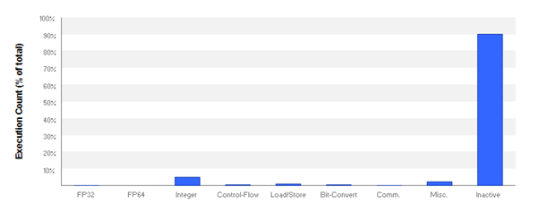
Obviously, there is something wrong with Hughes et al.’s algorithm, or its implementation. According to the article [3], it should be faster than, or on par with Billeter et al.’s. Obviously, it isn’t. Inspection using the NVidia Visual Profiler shows that the threads are mainly (over 90%) ‘Inactive’, which explains its lack of performance.
Having read the articles referred to above, I decided to see if I myself could become world champion parallel stream compaction, by writing a new algorithm based on some ideas not found in the articles. So, could I be the new world champion? No. I got results in between Orange Owl’s and Spataro’s, but could not get any faster.
So, the software by Markus Billeter, Ola Olsson, and Ulf Assarsson is the fastest parallel stream compaction algorithm in the world, they are world champion stream compaction, and we have to first learn why exactly, before we can surpass it, if at all. The question that then is:
“What makes Billeter, Olsson, and Assarsson’s parallel stream compaction Cuda program at least 2x as fast as its competitors?
Next
The implementation of Billeter et al.’s algorithm is an optimized library. Optimized also with respect to maintenance: no duplicate code, which makes it fairly cryptic, thus hard to decipher its operational details. Next up is a general description of their program, and its main parameters. The algorithm has three main steps which will be discussed in subsequent posts. Along the way I hope to disclose why their code is at least twice as fast as the other algorithm implementations.
References
[1] Billeter M, Olsson O, Assarsson U: Efficient Stream Compaction on Wide SIMD Many-Core Architectures. In Proceedings of the Conference on High Performance Graphics Vol. 2009 (2009), p. 159-166.
New Orleans, Louisiana — August 01 – 03, 2009. ACM New York, NY, USA. (http://citeseerx.ist.psu.edu/viewdoc/download;jsessionid=4FE2F7D1EBA4C616804F53FEF5A95DE2?doi=10.1.1.152.6594&rep=rep1&type=pdf ).
[2] Spataro Davide: Stream Compaction on GPU – Efficient implementation – CUDA (Blog 23-05-2015: http://www.davidespataro.it/cuda-stream-compaction-efficient-implementation/ ).
[3] Hughes D.M. Lim I.S. Jones M.W. Knoll A. Spencer B.: InK-Compact: In-Kernel Stream Compaction and Its Application to
Multi-Kernel Data Visualization on General-Purpose GPUs. In: Computer Graphics Forum, Volume 32 Issue 6 September 2013 Pages 178 – 188. (https://github.com/tpn/pdfs/blob/master/InK-Compact-%20In-Kernel%20Stream%20Compaction%20and%20Its%20Application%20to%20Multi-Kernel%20Data%20Visualization%20on%20General-Purpose%20GPUs%20-%202013.pdf ).
[4] Source code Billeter, Olsson, and Assarsson: https://newq.net/archived/www.cse.chalmers.se/pub/pp/index.html .
[5] Source code Spataro: https://github.com/knotman90/cuStreamComp
[6] Source code Hughes, Lim, Jones, Knoll, and Spencer: https://sourceforge.net/projects/inkc/
[7] Cuda 8 (September 2016 release, includes Thrust): https://developer.nvidia.com/cuda-toolkit .
[8] Orange Owls Solutions implementation of Spataro’s: https://github.com/OrangeOwlSolutions/streamCompaction
For those interested: I have prepared three programs that experiment with the Cuda stream compaction implementions of Billeter et al., Spataro and Orange Owls. You can request download links (executables and sources) by creating a comment.

Hello Bytekitchen.
Interesting post :)! Perhaps a silly question: if we would do these tests on my Gigabyte GeForce GTX 1080, do you expect we get the same order in best to worst algorithms?
I would think so actually, but i can expect that the differences between them would be smaller?
Cheers!
Hey Cubey,
Thanks for the question!
Your GTX 1080 is of course a whole lot faster than my GTX 690. It is faster (among other reasons)because the hardware needs less time to perform the same operations. Therefore I think that the order in best to worst algorithms is preserved when running these programs on your card.
Your card is also faster because it has more processors. Timing differences will be smaller in absolute sense (of course), but I think by and large the relative relations between the processing times will hold. The difference in performance between our cards is, in the end, just that the work is done faster, and more of the work is done at the same time.
The critical question then is whether the relation between the performance times is a factor (as in multiplication of a by b) or additive (a difference as in a minus b). To illustrate, I’ve set up a table of processing times for various input sizes. The programs have been run for 1000 iterations on structured data (see post above), as release builds, without a debugger attached. Times are in milliseconds.
It is now clear that the algorithm by Billiter, Olsson, and Assarsson (BOA) is a *factor* (of about) 2 faster than the other two implementations. The relation between the implementations by Orange Owls and Spataro is additive (about 0.11 ms). So, the difference between BOA on the one hand and Orange Owl and Spataro on the other hand will always be meaningful.
Hello Marc,
thank you for this comprehensive reply! Quite insightful. I agree with your statements. So independent on the workload (input length) or GPU used the difference in factor between BOA on the one hand and Orange Owls / Spataro on the other hand will remain about the same. Right?
Cheers, Cubey
Hi Qubey,
Your conclusion seems over-enthusiastic. So there is something wrong with my answer to your original question.
Forget the answer above. We are going to do this thoroughly, and along a different line. Your question is important: if I select an algorithm on my current hardware, I also want it to be the correct choice on my next graphics card, right?
Let’s experiment. I will provide a few programs that allow for experimentation with the software of BOA, Spataro, and Orange Owls on graphics cards of the same generation as my graphics card and later. I will make this software publicly available, anyone can experiment (at his or her own risk, I will add a license). The programs just add an execution context, so anybody can experiment without programming. I will also add the source code.
Do you still have your previous graphics card? Is it an Nvidia card? If so, what type is it? May be we could also enter that card into the experimentation too?
Let’s experiment, collect the results, and present them in a next blog post.
Hello Marc,
indeed, that is perhaps the important question: is a current choice or algorithm based on a current system if one would upgrade the graphic card?
Yes, let us experiment! I think i still got my old graphic card stored away in a drawer somewhere… an Nvidia GTX 580.
Additionally, i have another system standing here with a Nvidia GTX 660 installed.
An Asus GTX960 is also laying around here, which still needs to be put in the system where the 660 is currently installed.
If the software packages are also backwards compatible, then we could also include my dads pc with an Nvidia GTX 480.
As you said: let’s experiment and collect the results!
Hi Cubey,
The implementations by Spataro and Orange Owls use intrisics that are available from the Kepler architecture onward only. So the 580 and the 480 cards cannot participate in the comparison (sorry). On the other hand, the 660, the 960, and the 1080 are great!