Vector –Matrix Inner Product with Computer Shader and C++ AMP
Large vector-matrix inner products by the GPU are 250 times faster than straight forward CPU implementations on my PC. Using C++ AMP or a Compute Shader the GPU realized a performance of over 30 gFLOPS. That is a huge increase, but my GPU has a “computational power” (whatever that may be) of 1 teraFLOP, and 30 gFLOPS is still a long way from 1000 gFLOPS.
This article presents a general architectural view of the GPU and some details of a particular exemplar: the Ati Radeon HD5750. Then code examples follow that show various approaches to large vector-matrix products. Of course the algorithms at the end of the article are the fastest. It is also the simplest.
Unified View of the GPU Architecture
Programming the GPU is based on an architectural view of the GPU. The purpose of this architectural view is to provide a unified perspective on GPUs from various vendors, hence with different hardware setup. It is this unified architecture that’s being programmed against using DirectX11. A good source of information on Direct Compute and Compute Shaders is the Microsoft Direct Compute BLog. The architecture described below is based on information from Chas Boyd’s talk at PDC09, as published on Channel9. Of course, this blog post only presents some fragments of the information found there.
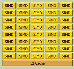
A GPU is considered to be build from a number of SIMD cores. SIMD means: Single Instruction Multiple Data. By the way, the pictures below are hyperlinks to their source.
The idea is that a single instruction is executed on a lot of data, in parallel. The SIMD processing unit is particularly fit for “data parallel” algorithms. A GPU may consist of 32 SIMD cores (yes, the image shows 40 cores) that access memory with 32 floats at a time (128 bit bus width). Typically the processor runs at 1Ghz, and has a (theoretical) computational power of about 1 TeraFLOP.
A SIMD core uses several kinds of memory:
- 16 Kbyte of (32-bit) registers. Used for local variables
- 8 Kbyte SIMD shared memory, L1 cache.
- L2 cache
The GPU as a whole has typically 1Gb of general RAM. Memory access bandwidth is typically of order 100GBit/s.
Programming Model
A GPU is programmed using a Compute Shader or C++ AMP. Developers can write compute shaders in HLSL (Looks like C) to be executed on the GPU. AMD is a C++ library. The GPU can run up to 1024 threads per SIMD. A thread is a line of execution through code. The SIMD shared memory is shared among the threads of a SIMD. It is programmable in the sense that you can declare variables (arrays) as “groupshared” and they will be stored in the Local Data Share. Note however, that over-allocation will spill the variables to general RAM, thus reducing performance. Local variables in shader code will be stored in registers.
Tactics
The GPU architecture suggests programming tactics that will optimize performance.
- Do your program logic on the CPU, send the data to the GPU for operations that apply to (about) all of the data and contain a minimal number of alternative processing paths.
- Load as much data as possible into the GPU general RAM, so as to prevent the GPU waiting for data from CPU memory.
- Declare registers to store isolated local variables
- Cache data that you reuse in “groupshared” Memory. Don’t cache data you don’t reuse. Keep in mind that you can share cached data among the threads of a single group only.
- Use as much threads as possible. This requires you use only small amounts of cache memory per thread.
- Utilize the GPU as efficiently as possible by offering much more threads to it than it can process in a small amount of time.
- Plan the use of threads and memory ahead, then experiment to optimize.
Loading data from CPU memory into GPU memory passes the PCIe bridge which has a bandwidth, typically of order 1GBit/s; that is, it is a bottleneck.
So, you really like to load as much data onto GPU memory before executing your code.
The trick in planning your parallelism is to chop up (schedule, that is J ) the work in SIMD size chunks. You can declare groups of threads; the size of the groups and the number of groups. A group is typically executed by a single SIMD. To optimize performance, use Group Shared Memory, and set up the memory consumption of your thread group so it will fit into the available Group Shared Memory. That is: restrict the number of threads per group, and make sure you have a sufficient number of groups. Thread groups are three dimensional. My hypothesis at this time is that it is best to fit the dimensionality of the thread groups to match the structure of the end result. More about this below. Synchronization of the threads within a thread group flushes the GroupShared Memory of the SIMD.
A register typically has a lifetime that is bound to a thread. Individual threads are member of several groups – depending on how you program stuff. So, intermediate results aggregated by thread groups can be stored in registers.
Does My ATI Radeon HD5750 GPU Look Like This Architecture… A Bit?
The picture below (from here) is of the HD5770, which has 10 SIMD cores, one more than the HD5750.
What do we see here?
- SIMD engines. We see 10 cores for the HD5770, but there are 9 in the HD5750. Each core consists of 16 red blocks (streaming cores) and 4 yellow blocks (texture units).
- Registers (light red lines between the red blocks).
- L1 Textures caches, 18Kbyte per SIMD.
- Local Data Share, 32 Kbyte per SIMD.
- L2 caches, 8 Kbyte each.
Not visible is the 1Gb general RAM.
The processing unit runs at 700Mhz, memory runs at 1,150Mhz. Over clocking is possible however. The computational power is 1,008 TeraFLOP. Memory bandwidth is 73.6 GBit/s.
So, my GPU is quite a lot less powerful than the reference model. At first, a bit disappointing but on the other hand: much software I write for this GPU cannot run on the PCs of most people I know – their PCs are too old.
Various Approaches to Vector-Matrix Multiplication
Below we will see a number of approaches to vector-matrix multiplication discussed. The will include measurements of time and capacity. So, how do we execute the code and what do we measure?
Times measured include a number of iterations that each multiply the vector by the matrix. Usually this is 100 iterations, but fast alternatives get 1000 iterations. The faster the alternative, the more we are interested in variance and overhead.
Measurements:
- Do not include data upload and download times.
- Concern an equal data load, 12,288 input elements if the alternative can handle it.
- Correctness check; computation is also performed by CPU code, reference code.
- Run a release build from Visual Studio, without debugging.
- Allow AMP programs get a warming up run.
Vector-Matrix Product by CPU: Reference Measurement
In order to determine the performance gain, we measure the time it takes the CPU to perform the product. The algorithm, hence the code is straightforward:
In this particular case rows = cols = 12,288. The average over 100 runs is 2,452 ms, or 2.45 seconds. This amounts to a time performance of 0.12 gFLOPS (giga FLOPS: FLoating point Operations Per Second). We restrict floating point operations to addition and multiplication (yes, that includes subtraction and division). We calculate gFLOPS as:
2 / ms x Rows / 1000 x Cols / 1000, where ms is the average time in milliseconds.
The result of the test is correct.
Parallel Patterns Library
Although this blog post is about GPU performance, I took a quick look at PPL performance. We then see a performance gain of a factor 2, but the result is incorrect, that is, the above code leads to indeterminacy in a parallel_for loop. I left it at that, for now.
Matrix-Matrix Product
We can of course, view a vector as a matrix with a single column. The C++ AMP documentation has a running code example of a matrix multiplication. There is also an accompanying compute shader analog.
AMP
To the standard AMP example I’ve added some optimizing changes, and measured the performance. The AMP code look like this:
Here: amp is an alias for the Concurrency namespace. The tile size TS has been set to 32, which is the maximum; the product of the dimensional extents of a compute domain should not exceed 1024. The extent of the compute domain has been changed to depend on B, the matrix, instead of the output vector. The loop that sums element products has been unrolled in order to further improve performance.
As mentioned above, we start with a warming up. As is clear from the code we do not measure data transport to and from the GPU. Time measurements are over 100 iterations. The average run time obtained is 9,266.6 ms, hence 0.01 gFLOPS. The result after the test run was correct.
The data load is limited to 7*1024 = 7,168; that is 8*1024 is unstable.
Compute Shader
The above code was adapted to also run as a compute shader. The code looks like this:
The variables Group_SIZE_X and Group_SIZE_Y are passed into the shader at compile time, and are set to 32 each.
Time measurements are over 100 iterations. The average run time obtained is 11,468.3 ms, hence 0.01 gFLOPS. The result after the test run was correct. The data load is limited to 7*1024 = 7,168; that is 8*1024 is unstable.
Analysis
The performance of the compute shader is slightly worse that the AMP variant. Analysis with the Visual Studio 11 Concurrency Visualizer shows that work by the GPU in case of the compute shader program is executes in small spurts, separated by small periods of idleness, whereas in the AMP program the work is executed by the GPU in one contiguous period of time.
Nevertheless, performance is bad, worse than the CPU alternative. Why? Take a look at the picture below:
For any value of t_idx.global[0] – which is based on the extent of the matrix- that is unequal to zero, vector A does not have a value. So, in fact, if N is the number of elements in the vector, we do O( N3)retrievals but only O(N2) computations. So, we need an algorithm that is based on the extent of a vector, say the output vector.
Vector-Matrix Product
Somehow, it proved easier to develop the vector-matrix product as a compute shader. This is in spite of the fact that unlike AMP, it is not possible (yet?) to trace a running compute shader in Visual Studio. The idea of the algorithm is that we tile the vector in one dimension, and the matrix in two, thus obtaining the effect that the vector tile can be reused in multiplications with the matrix tile.
Compute Shader
A new compute shader was developed. This compute shader caches vector and matrix data in Group Shared memory. The HLSL code looks like this:
This program can handle much larger amounts of data. Indeed, this program runs problem free for a vector of 12,288 elements and a total data size of 576 Mbyte. Using an input vector of 12,288 elements, with total data size of 576 Mbyte. The time performance is 10.3 ms per run, averaged over 1,000 runs, which amounts to 29.3 gFLOPS. The result of the final run was reported to be correct.
AMP
In analogy to the compute shader above I wrote (and borrowed 🙂 ) a C++ AMP program. The main method looks like this:
The matrix is a vector with size * size elements. He tile size was chosen to be 128, because that setting yields optimal performance. The program was run on an input vector of 12,288 elements again, with total data size of 576 Mbyte. The time performance is 10.1 ms per run, averaged over 1000 runs, which amounts to 30.0 gFLOPS. The result of the final run was reported to be correct.
Analysis
We see here that the performance has much improved. When compared to the reference case, we can now do it (in milliseconds) 2,452 : 10.1 = 243 : 1, hence 243 times faster.
Simpler
Then, I read an MSDN Magazine article on AMP tiling by Daniel Moth, and it reminded me that caching is useless if you do not reuse the data. Well, the above algorithm does not reuse the cached matrix data. So I adapted the Compute Shader program to retrieve matrix data from central GPU memory directly. The HLSL code looks like this:
Note the tileSize of 512(!). This program was run for a vector of 12,288 elements and a total data size of 576 Mbyte. The time performance is again 10.3 ms for a multiplication which amounts to 29,3 gFLOPS (averaged over 1000 runs). The result of the final run was reported to be correct. So, indeed, caching the matrix data does not add any performance improvement.
AMP
For completeness, the AMP version:
Time performance is optimal for a tile size of 128, in case the number of vector elements is 12,288. We obtain an average run time of 9.7 ms (averaged over 1,000 runs), and a corresponding 31.1 gFLOPS. The result of the final run was correct. This program is 2452 / 9.7 = 252.8 times as fast as the reference implementation.
Conclusions
Developing an algorithm for vector-matrix inner product has demonstrated comparable performance for Compute Shaders and AMP, but much better tooling support for AMP: we can step through AMP code while debugging, and the Concurrency Visualizer has an AMP line. This better tool support helped very well in analyzing performance of a first shot at the algorithm. The final algorithm proved over 250 times faster than a straight forward CPU program for the same functionality.
Detailed knowledge of the GPU architecture, or the hardware model, proved of limited value. When trying to run the program with either the maximum nr of threads per group, or the maximum amount of data per Group Shared Memory, I ran into parameter value limits, instabilities, performance loss, and incorrect results. I guess, you will have to leave the detailed optimization to the GPU driver and to the AMP compiler.
One question keeps bothering me though: Where is my TeraFLOP?
I mean, Direct Compute was introduced with the slogan “A teraFLOP for every one of us”, AMP is built on top of Direct Compute, and my GPU has a computational power of 1.08 TeraFLOP. Am I not ‘one of us’?


