Data Compression for the Kinect

Transmitting uncompressed Kinect depth and color data requires a network bandwidth of about 460Mbit/s. Using the RleCodec or the LZ4 library we achieve tremendous compression – a compression ratio of 10 or 22 respectively, at lightning speed – over 1600Mbytes/s. We achieve this not so much by the compression algorithms, but by removing undesirable effects (jitter, by the DiscreteMedianFilter) and redundancy (already sent data, by taking the Delta).

Introduction

From the start, one goal of the Kinect Client Server (KCS) project was to provide a version of the KCS viewer, called 3D-TV, from the Windows Store. Because of certification requirement 3.1 (V5.0)

“Windows Store apps must not communicate with local desktop applications or services via local mechanisms,..”

3D-TV has to connect to a KinectColorDepth server application on another PC. In practice, the network bandwidth that is required to transfer uncompressed Kinect depth and color data over Ethernet LAN using TCP is about 460Mbit/s, see e.g. the blog post on the jitter filter. This is a lot, and we would like to reduce it using data compression.

This is the final post in a series of three on the Kinect Client Server system, an Open Source project at CodePlex, where the source code of the software discussed here can be obtained.

What Do We Need?

Let’s first clarify the units of measurements we use.

Mega and Giga

There is some confusion regarding the terms Mega and Giga, as in Megabit.

• For files 1 Megabit = 2^20 bits, and 1 Gigabit = 2^30 bits.
• For network bandwidth, 1 megabit = 10^6 bits, and 1 gigabit = 10^9 bits.

Here we will use the units for network bandwidth. The Kinect produces a color frame of 4 bytes and a depth frame of 2 bytes at 30 frames per second. This amounts to:

30 FPS x 640×48 resolution x (2 depth bytes + 4 color bytes) x 8 bits = 442.4 Mbit/s = 55.3 Mbyte/s.

We have seen before that the actual network bandwidth is about 460Mbit/s, so network transport creates about 18Mbit/s overhead, or about 4%.

Since we are dealing with data here that is streamed at 30 FPS, time performance is more important than compression rate. It turns out that a compression rate of at least 2 (compressed file size is at most 50% of uncompressed size), in about 5ms satisfies all requirements.

Data Compression: Background, Existing Solutions

Theory

If you are looking for an introduction to data compression, you might want to take a look at Rui del-Negro’s excellent 3 part introduction to data compression. In short: there are lossless compression techniques and lossy compression techniques. The lossy ones achieve better compression, but at the expense of some loss of the original data. This loss can be a nuisance, or irrelevant, e.g. because it defines information that cannot be detected by our senses. Both types of compression are applied, often in combination, to images, video and sound.

The simplest compression technique is Run Length Encoding, a lossless compression technique. It simply replaces a sequence of identical tokens by one occurrence of the token and the count of occurrences. A very popular somewhat more complex family of compression techniques is the LZ (Lempel-Ziv) family (e.g. LZ, LZ77, LZ78, LZW) which is a dictionary based, lossless compression. For video, the MPEG family of codecs is a well known solution.

Existing Solutions

There are many, many data compression libraries, see e.g. Stephan Busch’s Squeeze Chart for an overview and bench marks. Before I decided to roll my own implementation of a compression algorithm, I checked out two other solutions: The Windows Media Codecs In Window Media Foundation. But consider the following fragment from the Windows Media Codecs documentation:

It seems as if the codecs are way too slow: max 8Mbit/s where we need 442Mbit/s. The WMF codecs obviously serve a different purpose.

The compression used for higher compression levels seems primarily of the lossy type. Since we have only 640×480 pixels I’m not sure whether it is a good idea to go ‘lossy’. It also seems that not all versions of Windows 8 support the WMF.

LZ4, an open source compression library. This is a very fast compression library, see image below, from the website:

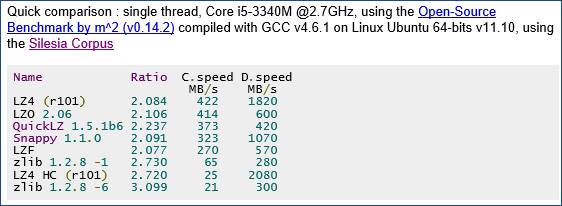
So, LZ4 can compress a file to 50% at over 400MByte/s. That is absolutely great! I’ve downloaded the source and tried it on Kinect color and depth data. Results are shown and compared in the Performance section.

The RleCodec

I decided to write my own data compression codec, and chose the Run Length Encoding algorithm as a starting point. Why?

Well, I expected a custom algorithm, tailored to the situation at hand would outperform the general purpose LZ4 library. And the assumption turned out to be correct. A prototype implementation of the RleCodec supported by both the DiscreteMedianFilter and creating a Delta before compressing data really outperformed the LZ4 reference implementation, as can be read from the performance data in the Performance section.

It only dawned on me much later that removing undesired effects (like jitter, by the DiscreteMedianFilter) and redundant information (already sent data, by taking the Delta) before compressing and transmitting data is not an improvement of just the RLE algorithm, but should be applied before any compression and transmission takes place. So, I adjusted my approach and in the performance comparison below, we compare the core RLE and LZ4 algorithms, and see that LZ4 is indeed the better algorithm.

However, I expect that in time the data compression codec will be implemented as a GPU program, because there might be other image pre-processing steps that will also have to be executed at the GPU on the server machine; to copy the data to the GPU just for compression requires too much overhead. It seems to me that for GPU implementations the RLE algorithm will turn out the better choice. The LZ4 algorithm is a dictionary based algorithm, and creating and consulting a dictionary requires intensive interaction with global memory on the GPU, which is relatively expensive. An algorithm that can do its computations purely locally has an advantage.

Design

Lossless or Lossy

Shall we call the RleCodec a lossy or lossless compression codec? Of course, RLE is lossless, but when compressing the data, the KinectColorDepth server also applies the DiscreteMedianFilter and takes the Delta with the previous frame. Both reduce the information contained in the data. Since these steps are responsible for enormous reduction of compressed size, I am inclined to consider the resulting library a lossy compression library, noting that it only looses information we would like to lose, i.e. the jitter and data we already sent over the wire.

Implementation

Algorithm

In compressing, transmitting, and decompressing data the KinectColorDepth server application takes the following steps:

1. Apply the DiscreteMedianFilter.
2. Take the Delta of the current input with the previous input.
3. Compress the data.
4. Transmit the data over Ethernet using TCP.
5. Decompress the data at the client side.
6. Update the previous frame with the Delta.

Since the first frame has no predecessor, it is a Delta itself and send over the network as a whole.

Code

The RleCodec was implemented in C++ as a template class. Like with the DiscreteMedianFilter, traits classes have been defined to inject the properties that are specific to color and depth data at compile time.

The interface consists of:

• A declaration that take the value type as the template argument.
• A constructor that takes the number of elements (not the number of bytes) as an argument.
• The size method that returns the byte size of the compressed data.
• The data method that returns a shared_ptr to the compressed data.
• The encode method that takes a vector of the data to compress, and stores the result in a private array.
• The decode method that takes a vector, of sufficient size, to write the decompressed data into.

Like the DiscreteMedianFilter, the RleCodec uses channels and an offset to control the level of parallelism and to skip channels that do not contain information (specifically, the A (alpha or opacity) channel of the color data). Parallelism is implemented using concurrency::parallel_for from the PPL library.

Meta Programming

The RleCodec contains some meta programming in the form of template classes that roll out loops over the channels and offset during compilation. The idea is that removing logic that loops over channels and checks if a specific channel has to be processed or skipped will provide a performance gain. However, it turned out that this gain is only marginal (and a really thin margin 🙂 ). It seems as if the compiler obviates meta programming, except perhaps for very complicated cases.

Performance

How does our custom RLE codec perform in test environment and in the practice of transmitting Kinect data over a network? How does its performance compare to that of LZ4?. Let’s find out.

In Vitro Performance

In vitro performance tests evaluate in controlled and comparable circumstances the speed at which the algorithms compress and decompress data.

Timing

In order to get comparable timings for the two codecs, we measure the performance within the context of a small test program I wrote, the same program is used for both codecs. This makes the results comparable and sheds light on the usefulness of the codec in the context of transmitting Kinect data over a network.

Algorithm

In comparing the RleCodec and LZ4, both algorithms take advantage of working the delta of the input with the previous input. We use 3 subsequent depth frames and 3 subsequent color frames for a depth test and a color test. In a test the frames are processed following the sequence below:

1. Compute delta of current frame from previous frame.
2. Compress the delta.
3. Measure the time it takes to compress the delta
4. Decompress the delta
5. Measure the time it takes to decompress the delta
6. Update previous frame with the delta
7. Check correctness, i.e. the equality of the current input with the updated previous input.

We run the sequence 1000 times and average the results. Averaging is useful for processing times, the compression factor will be the same in each run. The frames we used are not filtered (DiscreteMedianFilter).

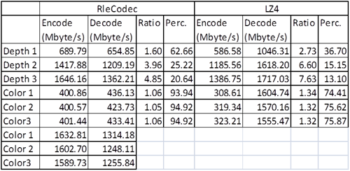
Let’s first establish that the performance of these libraries are of very different order than the performance of the WMF codecs. Let’s also establish that compression speed and decompression speed is much more than sufficient: as noted above 50Mbyte/s would do.

For depth data, we see that the RleCodec delivers fastest compression. LZ4 delivers faster decompression, and obtains stronger compression.

The RleCodec was tested twice with the color data. In the first test we interpreted the color data as of type unsigned char. We used 3 channels with offset 4 to compress it. In the second test we interpreted the color data as unsigned int. We used 4 channels, with offset 4. We see that now the RleCodec runs about 4 times as fast as with char data. The compression strength is the same, however. So, for color data, the same picture arises as with depth data: times are of the same order, but LZ4 creates stronger compression.

The difference in naked compression ratios has limited relevance, however. We will see in the section on In Vivo testing that the effects of working with a Delta, an in particular of the DiscreteMedianFilter dwarfs these differences.

We note that the first depth frame yields lesser results both for time performance and compression ratio. The lesser (de)compression speed is due to the initialization of the PPL concurrency library. The lesser compression ratio is illustrative of the effect of processing a Delta: the first frame has no predecessor, hence there is no Delta and the full frame is compressed. The second frame does have a Delta, and the compression ratio improves by a factor of 2.4 – 2.5.

In Vivo Performance

In Vivo tests measure, in fact, the effect of the DiscreteMedianFilter on the data compression. In Vivo performance testing measures the required network bandwidth in various configurations:

1. No compression, no filter (DiscreteMedianFilter).
2. With compression, no filter.
3. With compression, with filter, with noise.
4. With compression, with filter, without noise.

We measure the use of the RleCodec and the LZ4 libraries. Measurements are made for a static scene. Measuring means here to read values from the Task Manager’s Performance tab (update speed = low).

Using a static scene is looking for rock bottom results. Since activity in the scene- people moving around can be expressed as a noise level, resulting compression will always be somewhere between the noiseless level and the “no compression, no filter” level. Increase will be about linear, given the definition of noise as a percentage of changed pixels.

The measurements in the table below are in Megabits per second, whereas the table above shows measurements in Megabytes per second. So, in order to compare the numbers, if so required, the entries in the table below have to be divided by 8. Note that 460Mbit/s is 57.5Mbyte/s.

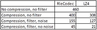
What we see is that:

• Compression of the delta reduces network bandwidth width 13* (RLE), or 33% (LZ4).
• Application of the filter reduces it further with 53% (RLE), or 39% (LZ4).
• Cancelling noise reduces it further with 24% (RLE), or 23% (LZ4).
• We end up with a compression factor of about 10 (RLE), or 22 (LZ4).

:-).

What do we transmit at the no noise level? Just the jitter beyond the breadth of the DiscreteMedianFilter, a lot of zeroes, and some networking overhead.

As noted above, the differences between the core RleCodec and LZ4 are insignificant compared to the effects of the DiscreteMedianFilter and taking the Delta.

Conclusions

Using the RleCodec or the LZ4 library we achieve tremendous compression, a compression ratio of 10 or 22 respectively , at lightning speed – over 1600Mbytes/s. We achieve this not so much by the compression algorithms, but by removing undesirable effects (jitter, by the DiscreteMedianFilter) and redundancy (already sent data, by taking the Delta).

ToDo

There is always more to wish for, so what more do we want?

Navigation needs to be improved. At the moment it is somewhat jerky because of the reduction in depth information. If we periodically, say once a second, send a full (delta yes, filter no) frame, in order to have all information at the client’s end, we might remedy this effect.

A GPU implementation. Compute shader or C++ AMP based. But only in combination with other processing steps that really need the GPU.

Improve on RLE. RLE compresses only sequences of the same token. What would it take to store each literal only once, and insert a reference to the first occurrence at reencountering it? Or would that be reinventing LZ?

A Jitter Filter for the Kinect

This blog post introduces a filter for the jitter caused by the Kinect depth sensor. The filter works essentially by applying a dynamic threshold. Experience shows that a threshold works much better than averaging, which has the disadvantage of negatively influencing motion detection, and has only moderate results. The presented DiscreteMedianFilter removes the jitter. A problem that remains to be solved is the manifestation of depth shadows. Performance of the filter is fine. Performance is great in the absence of depth shadow countermeasures.

Introduction

Kinect depth images show considerable jitter, see e.g. the depth samples from the SDK. Jitter degrades image quality. But it also makes compression(Run Length Encoding) harder; compression for the Kinect Server System will be discussed in a separate blog post. For these reasons we want to reduce the jitter, if not eliminate it.

Kinect Depth Data

What are the characteristics of Kinect depth data?

Literature on Statistical Analysis of the Depth Sensor

Internet search delivers a number of papers reporting on thorough analysis of the depth sensor. In particular:

[1] A very extensive and accessible technical report by M.R. Andersen, T. Jensen, P. Lisouski, A.K. Mortensen, M.K. Hansen, T. Gregersen and P. Ahrendt: Kinect Depth Sensor Evaluation for Computer Vision Applications.

[2] An also well readable article by Kourosh Khoshelham and Sander Oude Elberink.

[3] A more technically oriented article by Jae-Han Park, Yong-Deuk Shin, Ji-Hun Bae and Moon-Hong Baeg.

[4] Of course, there is always the Wikipedia

These articles discuss the Kinect 360. I’ve not found any evidence that these results do not carry over to the Kinect for Windows, within the range ([0.8m – 4m]) of the Default mode.

Depth Data

We are interested in the depth properties of the 640×480 spatial image that the Kinect produces at 30 FPS in the Default range. From the he SDK documentation we know that the Kinect provides depth measurements in millimeters. A dept value measures the distance between a coordinate in the spatial image and the corresponding coordinate in the parallel plane at the depth sensor, see image below from the Kinect SDK Documentation.

Some characteristics:

1. Spatial resolution: at 0.8m the 640×480 (width x height) depth coordinates cover an approximately 87cmx63cm plane. The resolution is inversely proportional with the squared distance from the depth sensor. The sensor has an angular field of view of 57° horizontally and 43° vertically.

2. Depth resolution: the real world distance between 2 subsequent depth values the Kinect can deliver is about 2mm at 1m from the Kinect, about 2.5cm at 3m, and about 7cm at 5m. Resolution decreases quadratically as a function of the distance.

Jitter

The Kinect depth measurements are characterized by some uncertainty that is expressible as a random error. One can distinguish between errors in the x,y-plane on the one hand, and on the z-axis (depth values) on the other hand. It is the latter that is referenced to as the depth jitter. The random error in the x,y-plane is much smaller than the depth jitter. I suspect it manifests itself as the color jitter in the KinectColorDepthServer through the mapping of color onto depth, but that still has to be sorted out. Nevertheless, the filter described here is also applied to the color data, after mapping onto depth.

The depth jitter has the following characteristics:

1. The error in depth measurements: The jitter is about a few millimeters at 0.5m, up to 4cm at 5m, increasing quadratically over the distance from the camera.

2. The jitter is a walk over a small number of nearby discrete values. We have already seen this in a previous post in The Byte Kitchen Blog, where we found a variance over mainly 3 different values, and incidentally 4 different values. Of course, for very long measuring times, we may expect an increased variance.

3. The jitter is much larger at the boundaries of depth shadows. Visually, this is a pretty disturbing effect, but the explanation is simple. The Kinect emits an infra red beam for depth measurements which, of course, creates a shadow. The jitter on the edges of a depth shadow jumps from an object to its shadow on the background which is usually much further away. We cannot remove this jitter without removing the difference between an object and its background, so for now, I’ve left it as is.

The miniature below is a link to a graph in [2] (page 1450, or 14 of 18) of the depth resolution (blue) and size of the theoretical depth measurement error (red).

 

A Kinect Produces a Limited Set of Discrete Depth Values

It is not the goal of the current project to correct the Kinect depth data, we just want to send it over an Ethernet network. What helps a lot is, and you could see this one coming:

The Kinect produces a limited set of depth values.

The Kinect for Windows produces 345 different depth values in the Default range, not counting the special values for unknown, and out of range measurements. The depth values for my Kinect for Windows are (divide by 8 to get the depth distance in mm):

This is the number of values for the Kinect for Windows. I also checked the number of unique values for my Kinect 360, and it has a larger but also stable set of unique depth values. The number of depth values is 781, due to the larger range.

The fact that a Kinect produces a limited and small set of depth values makes live a lot easier: we can use a lookup table were we would otherwise have to use function approximation. The availability of a lookup table is also good news for the time performance of the filter.

A question might be: can you use the depth table of an arbitrary Kinect to work with any other Kinect? I assume that each Kinect has a slightly different table, and this assumption is based on the fact that my Kinect for Windows has slightly different values than my Kinect 360, for the same sub range. However, if you use an upper bound search (this filter uses std::upper_bound), you will find the first value equal to or larger than a value from an arbitrary Kinect, which will usually be a working approximation (better than having the jitter). Of course, an adaptive table would be better, and it is on the ToDo list.

Design

I’ve experimented with several approaches: sliding window of temporal averages, Bilateral Filter. But these were unsatisfactory:

– Reduction of Jitter is much less good compared to applying a threshold.

– Movement detection is as much reduced as the jitter, which is an undesirable effect.

A simple threshold, of about the size of the breadth of the error function proved the best solution. As noted above, the jitter typically is limited to a few values above and below the ‘real’ value. We could call the ‘real’ value the median of the jitter range, and describe this jitter range not in terms of the depth values themselves but of the enumeration of the sorted list of discrete depth values (see table). We get a Discrete Median Filter if we map all discrete values within the range onto the median of that range (minding the asymmetry of the sub ranges at the boundaries of our sorted list).

The DiscreteMedianFilter Removes Jitter

In practice we see no jitter anymore when the filter is applied: The DiscreteMedianFilter ends the jitter (period). However, the filter is not applicable to (edges of) depth shadows.

Noise

Actually, it turned out that this filter is in fact too good. If the Kinect registers a moving object, we get a moving depth shadow. The filter cannot deal with illegal depth values, so we are stuck with a depth shadow smear.

A modest level of noise solves this problem. In each frame 10% of the pixels the filter skips is selected at random, and updated. This works fine, but it should be regarded as a temporal solution: the real problem is, of course, the depth shadow, and that should be taken up.

Implementation

The Discrete Median Filter was implemented in C++, as a template class, with a traits template class (struct, actually); one specialization for the depth value type and one specialization for the color value type, to set the parameters that are typical for each data type, and a policy template which holds the variant of the algorithm that is typical for the depth and color data respectively. For evaluation purposes, I also implemented traits and policy classes for unsigned int.

So, the DiscreteMedianFilter class is a template that takes a value type argument. Its interface consists of a parameter free constructor and the Filter method that takes a pointer to an input array and a pointer to a state. The method changes the state where the input deviates from the state more than a specified radius.

Channels and Offset

Color data is made up of RGBA data channels: e.g. R is a channel. Working with channels is inspired on data compression. More on this subject in the blog post on data compression.

The advantages of working with channels for the DiscreteMedianFilter are:

1. We can skip the A channel since it is all zeroes

2. Per channel, changes of color due to sensor errors are usually expressible as small changes, which is not the case for the color as a whole, so we get better filtering results.

3. There are less values: 3 x 256 vs 2^32, so the probability of equal values is higher.

Note that the more values are found to be within the range of values that do not need change, the better time performance we get.

The individual channels are not processed in parallel (unlike in the compression library). We will show below that parallelism should not be required (but actually is, as long as we have noise).

Code

The code is complex at points, so it seems to me that printing the code here would raise more questions than it would answer. Interested people may download the code from The Byte Kitchen Open Sources at Codeplex. If you have a question about the code, please post a comment.

Performance

How much space and time do we need for filtering?

A small test program was built to run the filter on a number of generated arrays simulating subsequent depth and color frames. The program size never gets over 25.4 megabytes. The processing speed (without noise) is:

– About 0.77ms for an array of 1228800 bytes (640×480=307200 ARGB color values); 1530Mbyte/s

– About 0.36ms for an array of 640×480=307200 unsigned short depth values; 1615Mbyte/s.

So, this is all very fast, on a relatively small footprint: in a little more than 1ms we have filtered both the depth and the color data of a Kinect frame.

The simple test program and its synthetic data are not suitable for use with noise. So, we measured the time the KinectColorDepthServer needs for calls to the DiscreteMedianFilter. In this case the noise is set at 10% of the values that would otherwise be skipped. The times below are averaged over 25,000 calls:

– Depth: 6.7ms per call.

– Color: 19.3ms per call.

So, we may conclude that the noise is really a performance killer. Another reason to tackle the depth shadow issue. Nevertheless, we are still within the 33ms time window that is available for each frame at 30 FPS.

Does the DiscreteMedianFilter has any effect on the required network capacity? No, in both cases a capacity of 460Mbit/s is required for a completely static scene, compression is off. I do have the impression that the filter has a smoothing effect on instantaneous (as opposed to average) required network capacity.

To do

There is always more to wish for, so what more do we want?

– Resolve the need for the noise factor, i.e. do something about the depth shadows. This will increase performance greatly.

– Because of filtering, navigation through the scene is jerky. There are much less depth values in the image, so movement is not so smooth. This is to be helped by sending a full depth image every now and then. After all, the filter only replaces values that differ more than a threshold, the rest of the image is retained. Refreshing the overall picture now and then retains the richness of the depth image, helps to make noise superfluous, and smoothes navigation.

– Make the table of depth values adaptive. If a value is not present we replace the nearest value. Of course, we would then also like to save the new table to file, and load it at any subsequent program starts.

Kinect Client Server System V0.2

The Kinect Client Server System V0.2 adds the possibility to V0.1 to watch Kinect Color and Depth data over a network, and to navigate the rendered 3D scene.

To support data transfer over TCP, the Kinect Client Server System (KCS system) contains a custom build implementation of Run Length Encoding compression.

To both maximize compression and improve image quality the KCS system uses a jitter filter

Introduction

Version 0.1 of the KCS system allowed the display of Kinect data in a Windows Store app. This is a restricted scenario: for security reasons, a Windows Store app cannot make a network connection to the same PC it is running on, unless in software development scenarios. Version 0.2 overcomes this restriction by:

1. Support for viewing Kinect data from another PC.

2. Providing the 3D-TV viewer from the Windows Store (free of charge).

Of course, V0.2 is an open Source project, the code and binaries can be downloaded from The Byte Kitchen’s open Source project at CodePlex.

Usage

The easiest way to start using the KCS system v0.2 is to download 3D-TV from the Windows Store, navigate to the Help-About screen (via the ‘Settings’ popup), click on the link to the online manual and follow the stepwise instructions.

The general usage schema is depicted below.

The PC called Kinect server runs the KinectColorDepthServer application. In order for the client PC running 3D-TV to find the server PC on the network, the server PC must be connected to gigabit Ethernet (cabled computer network, say) with a network adapter carrying the IP address 192.168.0.20. The IP address of the Ethernet adaptor of the PC running 3D-TV must satisfy 192.168.0.xxx, where 0 <= x <=255. It is wise to expect that required data capacity is well over 100Megabit/second.

The online manual also provides a complete description of the keyboard keys to be used for navigating around a Kinect scene.

More information

In a few more blog posts, I will discuss more technical details of the new features in the KCS system V0.2, specifically the jitter filter that is to stabilize the Kinect imagery and help in data compression, and the data compression itself.