CX Reconsidered [2]: MVVM to the Rescue

Tactical implementation of the MVVM pattern will stop CX constructs bleeding through all of your code. In the first installment of this series, I have argued that CX data and threading structures tend to proliferate throughout your program, and that this is both unlike advised & advertised by Microsoft and undesirable because it drives out the far better developed C++ constructs. What we need is development tactics that keep the CX layer as thin as possible. This blog post presents first steps in the development of such tactics aka software development patterns or practices.

The goal is that:

  1. CX is used within specific layers of the design of a program.
  2. Each CX layer has a very limited set responsibilities.
  3. CX can be put to good use for the assigned responsibilities.

This is the second blog post in a series of n about my experiences with CX, and how I intend to use it in working with C++ and Xaml in the context of Windows 8.The table of contents into that series can be found in the first article in this series.

Ok, at the end of part [1] I wrote that next up would be a review of a number of (heated) discussions around the introduction of CX. But I changed my mind. It seems to me that although there is definitely value in a well argued position, there is more value in a working solution. So, let’s take a look at a way to put CX at its proper place.

Advised & Advertised CX Usage Policy

The usage policy for CX is, according to MS employees and documentation, to limit the use of CX to a thin layer at the ABI boundary. See e.g. the first response of Herb Sutter in the discussion after this Build 2011 talk

[ABI: At the lowest level, the Windows Runtime consists of an application binary interface (ABI). The ABI is a binary contract that makes Windows Runtime APIs accessible to multiple programming languages such as JavaScript, the .NET languages, and Microsoft Visual C++. (from the Hilo documentation)]

So, when we are interacting with the environment of a Windows Store application or component, we have to deal with the ABI.

However, there is nothing inherent to CX to enforce the advised & advertised usage policy. In part [1] of this series, it has been argued that it is very hard to ‘escape’ from CX and to restrict CX to a thin ABI interface layer.

The main reason it is hard to escape CX is the approach to developing a native code program that is natural to Visual Studio. This approach is a copy of the approach to developing .Net applications. You choose a project template, which assigns a central position to the user interface, then you add functionality to the program, extending, so to say, the capabilities of the user interface. For Windows 8, MS has introduced this approach also for native code, and they call it working with C++/CX. Point is, it is not C++ at all. Note also that CX is far, far behind to .Net in its development.

Nonetheless, if you start development with a CX Visual Studio project, it is CX that is used to interact with WinRT, and it thus defines the interface to the environment of the program. Because CX defines the periphery of an application, a tendency arises to define the main data structures in CX as well as considering its execution thread, the UI thread, as the main flow of control. We tend to consider the UI thread as the main flow of control because today’s apps are typically architected to react to events in the application’s environment. A consequence of this design is that CX language constructs and data structures tend to proliferate throughout a program, to bleed through all of your code. This proliferation generates a number of problems:

  1. Non portable code. The code cannot be compiled with a non-MS compiler, hence is not fit for use on e.g. IOS or Android platforms.
  2. It drives out the far more developed and richer C++11 language constructs, idioms and data structures.
  3. It drives out the far better .Net developer experience, if we consider CX to be positioned as a native alternative to C# .Net.

So, since CX does not itself enforce the Advised and Advertised Usage Policy of confining CX to a thin ABI interface layer, it is the CX user that carries the burden.

As a CX user, you will need a software pattern that restricts CX to what it is good at (yes, it does have its strengths), and to locations where it is useful. Such restrictions can, of course, be realized by disciplined application of conventions, but here we strive to have structural constructs that support the desired restriction: structural constructs that put a definite end to CX proliferation.

In restricting the use of CX we assume the task to not define the main data structures in CX, and to not run the principle flow of control in CX. We are constructing a generally applicable, patterned approach to developing programs involving one thin ABI interface layer of CX.

Overview of the Solution

In this blog post we propose to implement MVVM as a double layered structure, as depicted in the diagram 1. Yes, layers can be expressed as rectangles (with rounded corners, even) as well.
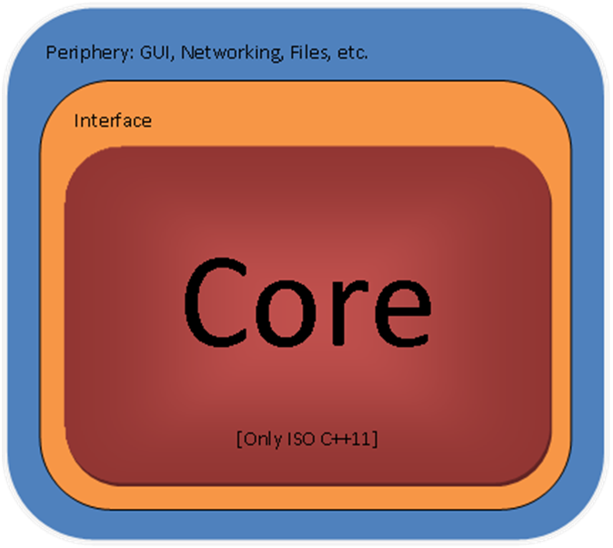
double layered Design

Diagram 1

As you can see, the core is considered the most important part of an application :-).

Components

In terms of physical components, or types of Visual Studio projects, or types of MS technologies, the proposal is to implement the core in C++, as a static library (or several static libraries); to implement the Interface as a WinRT Runtime Component written in CX; and to define the User Interface in Xaml with ‘code behind’ and other environmental interactions in preferably in C# or, if the situation necessitates the use of native code, in CX.

MVVM

The Model – View – ViewModel pattern will be used to stop the bleeding of CX constructs. Diagram 2 shows an image from the PRISM documentation that provides a very clear idea of the MVVM pattern.

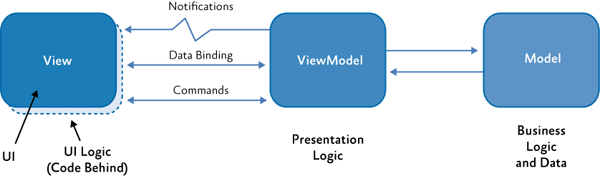
Diagram 2: PRISM interpretation of MVVM

In this article we will use a slight variation of MVVM: We consider the View to cover all of the environmental interactions, not just the GUI.

The MVVM pattern is tactically implemented as follows:

  • The View is realized in the Peripheral layer.
  • The ViewModel is realized in the Core layer.
  • The Model is also realized in the Core layer.

The Interface in Diagram 1 doesn’t have a specific role in the MVVM pattern, it has an implementational role.

Should you like to review the MVVM pattern, you might like to take a look at PRISM or the MVVM Light Toolkit (the historical roots of MVVM are really interesting as well).

The Peripheral Layer

Conforming to MVVM, we keep the Peripheral Layer as thin as possible. There are many different types of environmental interactions, which for now will be conveniently categorized as “The Xaml UI”, and “Other types of Environmental Interactions”.

The Xaml UI

There is always the discussion of how much code to allow in the code behind of an MVVM implementation. Since we really want layers that could contain CX to be thin, we decide two things:

  1. We use as little code in the user interface as possible. We limit the View to presenting data to the user, sending Commands and data to the ViewModel, and responding to events (callbacks) coming from the ViewModel. On the other hand, we allow code that defines interactions between user interface elements only. An example of the latter is opening a file picker when a user has clicked a button.
  2. We make the boundary between the Views on the one hand, and the ViewModels and Models on the other hand an ABI boundary.

Why an ABI boundary between View and ViewModel?

Well:

  1. For data binding and commanding. Any object exposed by a Windows Runtime Component across the ABI to a C# Xaml UI can be a source for data binding (this holds for C#, but not for CX).
  2. As a containment barrier in case a Xaml + CX GUI is used.

CX is Not a Good Choice For Xaml UI Code Behind

But that may change over time, of course, so let’s pin it down to “in august 2013”. So what’s wrong with the use of CX in the code behind of a Xaml UI?

  1. Data binding support is rather crude. Data binding in CX requires data binding source classes either to be decorated with the Bindable attribute or implement ICustomPropertyProvider, and have the bindable properties registered as ICustomProperties (see Nish Sivakumar’s implementation). Either requirement makes it extremely impractical (I would like to have written ‘impossible’ here) to data bind to properties exposed by a Windows Runtime Component. So, note that by requiring an ABI barrier between the UI and the ViewModel, we virtually ruled out CX as a possible language for Xaml code behind.
  2. MVVM support is unstable. I have defined several (non trivial) Xaml GUIs with CX as code behind platform, and seen the Xaml designer crash when a ViewModel locater class was inserted as a global resource to provide the DataContext and also data templates were provided to it as resources. On incidental beautifully sunny days the designer would provide an error message saying it could not instantiate some resource.
  3. Asynchronism: the PPL tasks library seems to have a special version for Windows Store applications, and it is rather hard to handle. It also frequently seems to operate not according to its documentation.

An argument to do use native code is performance. But we intend to keep the Views layer a thin layer, with an absolute minimum of functionality, so the performance of this layer will not easily affect general program performance. This is both because it is a minimal layer, and because it is the UI, i.e. it is about sending data about user actions to the core.

So, the performance argument has relatively little weight, and I think we are better off using C# .Net in the Views layer. Just because it supports development so much better. Think e.g. of the support for MVVM itself; there are several, and leading, MVVM frameworks to support you using the pattern for applications of arbitrary complexity.

When using C# in the code behind, one thing we do have to pay attention to though, is marshalling data across the ABI. We want data that crosses the ABI to be copied only if unavoidable or when we like to have a copy instead of the original. In general we want to have pointers (references) copied across the ABI. As we will see (elsewhere) this requires the use of write only data structures, also if we only want to read the data with which the write only data structure is initialized.

A possibly less urgent consideration is that the combination of a Xaml + C# GUI and native Windows Runtime Components is also a way to go on the Windows Phone platform.

Other Types of Environmental Interaction

The above section discusses the case for the Xaml UI – the View. How about the other types of environmental interaction mentioned, like database access, networking, file access, etc. Will you do that in .Net as well?

As a first go, yes. The peripheral layer should be minimal, so in the case of e.g. incoming network data you would like to stream incoming bytes as directly as possible into a buffer controlled by the core, as an unstructured stream of bytes. I think that we can set this up so that C# is used to control the work, but the system (written in native code) is used to do the work, hence performance will not be an issue.

If performance does turn out to be an issue (after measurements and analysis), I would use a native solution. Think of the C++ framework Casablanca, or even a custom solution in CX (indeed!).

The Core Layer

This is where we want to write static libraries of ISO C++11(+) only. Why?

C++11

Personally I happen to like C++ (and the STL), and version 11 more than earlier versions. Apart from that, maximum performance against minimal footprint gets you the most out of available hardware, which enriches user experience and hopefully also reduces (environmentally relevant) power consumption.

ISO: Portable Code

In the second quarter of 2013, some 44.4 million tablets were sold running either iOS, Android or Windows (8), of which 1.8 million are running Windows 8. In the same period, 227.3 million phones were sold running either Android, iOS or Windows Phone (8), of which 8.7 million are running Windows. So, we want to port our precious code to Android and iOS, thus reaching a market of say 271 million devices sold in the previous quarter alone; that’s over a billion in a year :-). And then there is also the PC market, of course, of about 500 million PCs running Windows, and coming to Windows 8 sooner or later.

Library

Putting code in a separate library allows you, among others, to specify the compile switches you need for a specific piece of source code. Using a library will allow us to specify that the compiler must not compile CX: we will not set the /ZW switch (or rather, we will set it to /ZW:nostdlib). So, CX constructs cannot bleed into such a library.

Static Library vs. Dynamic Load Library

Static libraries link at compile time, not at run time, hence have a relative performance advantage. Also if you export activatable classes (COM Components such as CX classes) from a static library, they cannot be activated. From a dynamic library, they can, see here. So, CX classes cannot be run from a static library.

Structured Data

We will make sure all main data structures are part of the Core Library. The use of system facilities, such as data transport, will be defined inside the core by C++ constructs, such as ‘pointer to stream’, that are used by the Interface layer to import and export the required data – as streams of primitive types. So, no CX owned main data structures.

Inversion of Control and Dependency Injection

We will expose any functionality only as Inversion of Control (IoC), also known as ‘The Hollywood Principle’: Don’t call us, we’ll call you, either by Dependency Injection (DI) or a Locator Service, see e.g. the articles by Martin Fowler here and here.

If the Core runs on its own thread(s), it is not susceptible to threading issues created by interactions with the Peripheral or Interface Layers (although it might have its own threading issues). We are also in a position to use STL threading; the bleeding of Microsoft threading technology into code we wish to be portable can be halted. So, no CX owned threads in the Core.

The Core and the UI: Ownership issues

We would like the Core library to be as independent as possible. The rationale behind these tactics is that independence from CX precludes having to incorporate CX constructs, either with respect to data or with respect to control. Another advantage may be that the Core’s lifecycle is not controlled from the UI thread, hence no freezing, throttling or killing. Of course, there is also no freezing of the UI.

The core library is already really independent by incorporating the program’s main data structures, by managing its own threads, and by utilizing the IoC pattern. Nevertheless, we can take independence a step further by looking at the ownership of the Core library. Who is the owner, that is: who controls its lifecycle?

The system starts up a Xaml application by calling the main method defined in App.g.hpp (CX) or App.g.i.cs (C#), which then starts up the UI. Usually you then instantiate other classes from the principal UI classes like the App or MainPage classes.

Alternatively you could define your own main method. The Xaml main method is decorated with the DISABLE_XAML_GENERATED_MAIN symbol. If that has been defined the decorated main function will not be used (surprise!). Your main method could instantiate the Core library and provide the UI with a handle, while holding a reference itself in order to control the lifecycle of the Core. The Core and the UI are now completely independent. An example of a system with an alternative main function is the demo application in the WinRT-Wrapper library by Tomas Pecholt. See here (the comment by Tomas) for an introduction to the WinRT-Wrapper.

Less invasive tactics (which I like better) may be to provide the library with a factory that creates the core, holds ownership and provides the UI with a ref counted handle. So, there is no ownership of the Core by the UI or the Interface.

First the Core

Where C# .Net applications start development at the UI, I think development in C++ + Xaml applications should start at the Core library.

The Interface Layer

Mediating between an application and the ABI, i.e. the system, that is where CX can be valuable. The strong point of CX is that it is ‘syntactic sugar’ over WRL constructs; CX reduces the amount of code markedly compared to the WRL. The WRL (the Windows Runtime Library, an ATL analogue), is itself intended to make interactions with the Windows Runtime practical. It has been shown multiple times (see specifically the articles by James McNellis) that CX makes it much more comfortable to interact with the Windows Runtime. If so required there is nevertheless always the possibility to pass by CX and insert some WRL code as demonstrated by James McNellis (see the answer) and here, and Kenny Kerr. As I understand it, CX code is the better choice for the bulk of WinRT interfacing code, but at times, WRL is the better choice for getting the ultimate performance. See the talk and slides by Sridhar Madhugiri at Build 2013

Since this is where CX is really useful, this is the first and foremost layer we want to keep thin. The layer’s responsibilities are (only) to relay data and commands across the ABI from the Peripheral Layer to the Core, vice versa. Of course, with a minimum of copy operations. We will use it, so to speak, to map the interface of the Core Library onto the ABI.

CX Reconsidered [1]: A Thin Layer of CX?

This is the first blog post in a series of n. The posts in this series will discuss opinions about C++/CX (from here on referred to as CX for reasons to be explained later), discuss pros and cons, and propose a meaningful way of working with C++ and Xaml in the context of Windows 8.The table of contents into that series will develop right below this sentence.

Part 1: A Thin Layer of CX? (this post).
Part 2: MVVM to the Rescue.
Part 3: Components on a thread

Introduction

Before Windows 8, I used to develop software in C# .Net for ASP.Net, WPF, and Silverlight, in C++ and some DirectX. What I needed was a better integration of C++, DirectX, and Xaml user interfaces. And low-and-behold, with Windows 8, Microsoft introduces CX. According to MS spokespeople CX is to be used as a thin layer around C++ programs, 99% of the code should be regular ISO C++. The value of the CX layer lies in the ability to cross the ABI (Application Binary Interface). The ABI is what makes it possible for programs written in language A to be used by programs written in language B. By the ABI, CX can also be provided with, among other things, a Xaml UI. Of course I jumped on it, this was exactly what I was looking for!

Now I’ve been writing software in CX (among others) since May 2012. It’s now June 2013, hence it is time to evaluate the experience; for myself, but hopefully this evaluation is of value to other developers too.

Conclusion

Let’s start with the conclusion, and then provide some analysis.

The conclusion is that I truly and intensely dislike CX. In the MS Forums (Fora?) someone wrote that programming the bare WinRT is tedious and rather painful. To me, the same holds for CX as well – although it is meant to relieve just that experience. My aversion for CX brought me to the point that I could not see where CX does come in handy, but thankfully I was able to put myself straight at that point.

What I dislike about CX can be summarized in 3 statements:

1. CX is supposed to be used as a thin layer, but escaping from CX is very hard. Once you start developing your program in it, you are likely forced to keep using it.

2. CX is not C++. That is, practices and idioms that you use with ISO C++11 are, as a rule, not valid for CX. This is why it is being called CX here, its native, but not C++.

3. CX is not C#. The same as above holds for C#, moreover, the developer experience with VS2012 is strongly inferior, as is the support for Xaml interfaces. Community contributions (such as MVVM light for .Net) are minimal.

That is, CX doesn’t meet your expectations as either a C++ developer or a C# developer. nor does it support ‘a thin layer of CX’ – it doesn’t let you go.

So, if you are a .Net developer that would like to author C++, doing CX is not the way to go.

Then there is this nagging question: If CX is meant to be used as only a thin layer around C++ code, then why has MS created the HILO example: a full-blown CX program? To show that CX should not be restricted to a thin layer?

Analysis

Why the aversion? Let’s go over the points in the Conclusion above.

A Thin layer of CX

The intention of a thin layer of CX is OK. It saves you the trouble of having to write code using the WRL (say COM). However, by the way MS has set application templates up that are based on CX, it is hard to restrain CX to a thin layer. A CX application has two powerful assets that bring it everywhere:

1. It defines the outer periphery of the application, that is all contact of the application with the world outside the application is via CX.

2. It runs on the main application thread; the UI thread, so it constitutes the main flow of control of the application.

This is a powerful combination in an application which architecture is to respond to environmental input and some system events. Anything coming from the environment: user input, file contents, network data, and data from files and databases, comes into the system in CX data structures, and on a CX thread.

Restrictions that apply to CX data structures tend to proliferate into user defined data types, and threading restrictions tend to proliferate into user spawned threads. Thus, the CX layer tends to expand. It will not be a thin layer, You will not work in C++, but in CX.

CX is not C++

If you are a C++ developer, you want to code in ISO C++11, not in CX, and certainly not in CX types instead of e.g. STL types. The developer experience of CX is strongly inferior to the C++ experience.

CX is not C#

C# .Net developers are used to a comfortable developer experience. Things tend to ‘just work’ (as they should). With CX, things don’t ‘just work’. Give a C# .Net developer the choice to switch to CX, and he/she will walk away smiling, if not grinning, after a short trial.

So, what happens is that CX hijacks your program, and you will have a hard time to escape. Once caught within CX you will be frustrated because you will be deprived of both the developer experience of both C++ and of C# .Net.

Not all is lost, however. With some architectural maneuvers, we will definitely put CX back in its cage! (But that will be in another installment in this series 🙂 ).

Next up: How CX was received in the forums (fora).

Harder to C++: Member Function Callbacks

Using a class member function as a callback is a possible source of confusion in C++, not in the least because C++11 brings considerable changes at this point. In this blog post we will see a few ways to do it well, and also mention deprecated facilities. It is not that I invented these techniques, but it seems helpful to spread the good word.

What is the Problem?

I wanted native C++ classes to report status updates to a XAML user interface. The XAML user interface has a method in its C++ code behind class that updates a TextBlock, and thus may inform the user about significant events in the program. The idea is to provide the objects of the native classes with a pointer or reference to the method in the code behind, so they can invoke that method and thus update the log.

How hard could that be??? Well, hard enough. So, I turned to the World Wide Web, and tried to find that one good solution. It turns out that C++ did not support callbacks in a very comfortable way until C++11, so easy to handle solutions are relatively new, and not easy to find on the World Wide Web. That’s why I wrote this blog post: to increase the probability that people needing to write callbacks for C++ can find a solution, if they need one. Note that if you need a systematic treatment of the subject you are probably better off by reading (parts of) an authoritative book e.g. “The C++ Standard Library”, by Nicolai M. Josuttis, 2nd ed.

This blog post will not in depth discuss the ins and outs of callbacks in general. Let’s just say that a callback is a function (or method) that is inserted into an object at runtime, such that the object may call the function whenever its logic dictates so. The object doesn’t know the definition of the injected function.

What’s the Solution?

The solution is to exploit a number of features that are new in C++11 and its Standard Template Library. Below we will see them introduced one by one, to settle in the end on a solution that seems most elegant and easy to use, to me (hopefully, you will agree with me on the conclusion). Note that the solutions presented here are simplified samples meant to demonstrate principle, not the code I use to log events to a display.

The ‘function’ Class

To conveniently create callable objects that are also easy to use, i.e. like standard C++ objects or functions, one uses the std::function class. For the samples in this blog post we will use the following function instantiation:

Variables of type WriteOutFunc are functions that take an int argument and return a string.

Below follows the definition of a simple class. Instantiations of this class will receive a function of type WriteOutFunc , and they will invoke (call) this function.

The method WriteForMe is there just for demonstration purposes. In real life the internal logic of a class dictates when the callback is invoked.

As a first use we instantiate a Caller, while injecting a lambda expression that implements a trivial roman number writer: it just writes the Roman number 3 (III). We do not yet inject a class member function, but just a lambda that is local to the _tmain function.

So what happens here is we initiate a Caller object with a simple lambda that returns “III”. Then we call the Caller’s method WriteForMe, with an argument ‘3’. Then WriteForMe invokes the lambda we injected and the result is returned by WriteForMe, and finally written to the standard out stream. The output is indeed “III” (without the quotes). All pretty standard.

The ‘bind’ Function

Next we define a Callee class that initiates a Caller object and injects a member function, so that the Caller object may invoke the method on this specific Callee object:

The important stuff is in the constructor. Since a member function is always called on a specific object, we ‘bind’ the object (this) to the member function WriteAsString, and assign the result to a WriteOutNumFunc variable m_numWriter. So, a call on m_numWriter(3) for a Callee my_callee is always my_callee ->WriteAsString(3). Once we have bound the Callee object and member function, we create a Caller object with the resulting WriteOutNumFunc object m_numWriter. The WriteForMe method is there again just to serve demonstration purposes.

The Callee class can be used as follows:

The output is 16 (not 12 🙂 ). I’ve added the offset, that gets modified when the callback is invoked by the Caller, and then added to the argument. This is to show that the Callee object can have its state changed by the Caller object by means of the callback. So, the Callee class demonstrates a solution to the problem how to create callbacks for class member functions. It’s a good solution, since it is built from STL facilities. It’s an elegant solution as well, it requires just a single extra line of code (bind) compared to the non member function case.

Let’s halt at this point for a moment, and discuss deprecated STL facilities. Point is that member function callbacks were, of course, already possible in C++ and the STL before C++11, but they were much more complex, and required much more work. See e.g. section 18.4.4.2 and 18.4.4.3 in Bjarne Stroustrup’s “The C++ programming Language, Special Edition”. Those sections lay out constructs that depend on templates as mem_fun and bind2nd. Point: these templates are now deprecated (see e.g. ‘Josuttis’, page 497).

In Comes the Lambda Expression

OK, we already have a neat solution to the problem posed. However, we can take it a bit further. We can introduce lambda expressions into the picture. With lambda expressions we can rewrite our Callee class as follows:

Well, this is considerably shorter, and works just as well. Of course, if you want to inject the same functionality into several objects, it is better to first create a named lambda expression, like so:

So, that’s it. And isn’t it a nice solution.

Harder to C++: Aligned Memory Allocation

Using the DirectX XMMatrix structure may under certain conditions crash your program. Overloading the new and delete operators in a specific way solves this problem, as does the STL aligned_storage class. This blog post integrates information from several sources – books, official documentation, forums / fora) to provide an overview of possible solutions.

What is the XMMatrix structure?

DirectX 11 is contains a high performance math library, called DirectXMath, specifically designed to handle up to 4 element vectors and up to 4 x 4 element matrices as fast as modern processors (implementing SSE2) can process them. XMVECTOR, and XMMATRIX are the central data structures in the library – you use them all through your code when programming DirectXMath.

In code you typically find something like

The function XMMatrixIdentity is also part of the library, along with a host of other functions, and generates an Identity matrix. For the uninitiated: multiplying a matrix A with an equal dimensioned identity matrix is like multiplying an integer by 1.

So, do we want to use XMMATRIX? Although there are other, similar data structures in the library? Yes, we do. We want the performance, the other data structures don’t offer the same performance, or the same compatibility with functions like XMMatrixIdentity.

What is the Problem, Exactly

Having decided we want to use XMVECTOR and XMMATRIX we will have to deal with the requirements for their use, which is that these structures need to be 16 byte aligned in memory (RAM). To be 16 byte aligned in memory means that the memory address of the data structure is a multiple of 16. The alignment requirement entails that any data structure that contains XMVECTOR or XMMATRIX also needs to be 16 byte aligned, etc. (recursively).

In many scenario’s in Windows 8 this is not a problem, you will not notice this requirement exists. However, I just happened to have stumbled upon a scenario in which the requirement does come to play, and it crashes my program.

The scenario is this: In a windows Store application (henceforth WinRT application) define a native class (pure C++, as opposed to C++/CX). holding an XMMATRIX object. This class’ constructor creates an XMMATRIX matrix and assigns an identity matrix to it using the XMMatrixIdentity function. In release builds (but not in debug builds) instantiating this class on the heap (not on the stack, and not as a static variable) will crash the program – every once in a while (!). So, for testing purposes I surrounded creation and destruction of an object of my class with a for loop. Within 10 iterations the program then practically always crashes.

The class looks like this.

And we use it in MainPage.cpp (this is about where you start programming a WinRT application) like this:

The error message looks like this, location 0xFFFFFFFF is typical for this error:

What is the Solution?

Of course, I could not be the only one that has encountered this problem, and indeed, a number of other people also got stuck. It turns out that people that come to a forum with a hard problem definitely find a lot of good intentions, though sometimes founded on arrogance. Alas they not that often find authoritative knowledge of C++ and the Standard Template Library, or even a clear understanding of their problem. Not that I myself am such an expert, but it is painful to browse through the numerous accounts that describe how a person went to the forum in despair with a problem he couldn’t solve or even understand, and subsequently had to fend off several guys that try to push very bad solutions onto him, and who typically end up fighting among each other which of them is really knowledgeable. It makes you think twice before asking for help.

Nevertheless, I managed to work my way through the debris, and find some valuable information. In this blog post we will examine three solutions from various sources:

  1. Use of _aligned_malloc and placement new by the MainPage class. This leaves the DXMathTrial class unchanged
  2. Overloading the new and delete operators of the DXMathTrial class.
  3. Creating an aligned typedef with the aligned_storage class

From the DirectXMath documentation we learn that we can overload the new and delete operators if we want to allocate 16 byte aligned variables on the heap of a class with XMMATRIX / XMVECTOR members. The documentation also suggests the use _aligned_malloc, see below. We can combine that nicely with placement new, see e.g. section 10.4.11, Special Edition of the good old C++ manual by Stroustrup. The latter idiom refers to a standard overload of the new operator that takes a memory address as an argument.

Placement new

What we do in this scenario, is we first allocate a correctly aligned block of memory with _aligned_malloc, then call placement new to construct an object of the DXMathTrial class at the obtained and aligned address. To destroy an object we first call the destructor of our DXMathTrial object, then free the allocated memory with _aligned_free. See the code below.

This solution works, and we have fine control over it: if we put the alignment to 8, we get the errors right back again. Nevertheless, this solution has some drawbacks: matter of style, or good taste.

  1. Although the DXMathTrial holds the XMMATRIX, the MainPage object has to do all the work to get the instantiation right. This is not really like the OO spirit, it doesn’t seem fair. The DXMathTrial class should hold the code to make instantiation of its objects easy and natural.
  2. It now takes much more code to create and delete an object: 7 lines instead of 2;

Overloading new  and delete

To alleviate the drawbacks of the above solution, one can overload the new and delete operators. This can be done globally (no!), or just for the relevant class.

But how does one overload new and delete? That is not straightforward, and I never did that before. Information about overloading new and delete in the context of memory alignment on the heap can be found e.g. here. Funny how the contributors do not mention XMMATRIX / XMVECTOR at all. So, you cannot find this solution on the internet using search terms describing your solution only, you will have to describe the solution!

Overloading new and delete is well treated in e.g. S.B. Lippman et all.: C++ Primer, Fifth Edition). It boils down to allocating memory in a user defined new operator overload, and de-allocating it in a user defined delete overload. In this case we will do the (de-) allocation with the ‘aligned’ variants, which gives us the following definition for the DXMathTrial class.

Testing with our initial definition of the MainPage class confirms that this is a solution. The drawbacks of the first solution are now gone, but we now see other drawbacks:

  • _aligned_malloc and _aligned_free are Microsoft specific; members of the VC++ CRT. We would prefer a solution that is completely general, one that is pure standard C++ & STL.
  • What I didn’t do here is overload all new and delete operators, but that really *is* required. That would make 8 overloads in all (see e.g. section 19.1.1 in S.B. Lippman et all.: C++ Primer, Fifth Edition). Code bloat!

The aligned_storage class

The Standard Template Library contains the aligned_storage class. It is a template that takes two value parameters: the size of the memory to be allocated, and the required alignment. To use it we add one line of code (!) to the DXMathTrial.h file to define an aligned version of the DXMathTrial class, which we will call DXMathTrialA (appending the ‘A’ may become a naming convention). We adapt our MainPage code accordingly. This gives us the following class:

With corresponding usage:

And now the problem has gone. Man, what a solution! …

BUT, aligned_storage requires the type to be aligned to be a POD type (see here for an explanation). The class above is at the edge of being a POD type. If you e.g. add a member method that sets m_matrix to the identity matrix, like so:

the problems are back again. So, we settle at overloading new and delete.

Inheritance and Membership Relations

The final question we would like to see answered is to what extent the solution involving overloaded new and delete operators propagates through membership and inheritance relations. To that end we define a class A_Base, and A_Child that both contain an XMMATRIX member, and both assign the identity matrix to this member in a dedicated method. A pointer to class A_Child will be a member of the DXMathTrial class, and allocation will be on the heap. The classes look like this.

Note that the definition of the overloaded operators have been simplified (past sound programming practice). The usage of the DXMathTrial class is unchanged. The result is that no exceptions are thrown. So, the new and delete operators of member classes also need to be overridden, but it suffices to overload these operators in the base class. This then is the solution.

My Home-Based Web and Mail Server: Gone!

At home I had a server that hosted my company’s website and the mail server that processed mail directed at (me at) my company. A nice small Windows 2008 server that was always on, never crashed, never had any other problems, always correctly finished its backup, it just did its job. Implemented on my old (2002, I think) Dell 360 Workstation. The only problem we had with it was that it had to be close to the ADSL connection which is next to our dinner table. The Dell 360 is a relatively silent computer, but, you can hear it, and after a few years (to me, for some family members it was already after a few months) the noise gets annoying, and changes have to be made.

One of the joys of a home-based server, on an old pc, is that it is free: no costs are involved except for some electricity. So, the challenge became to replace the home-based server with a solution that is also free, or almost free. So that is what this blog post is really about. How can you get basic IT facilities for your home-based startup company (almost) for free. Home-based means, among other things, that internet access already exists.

So, let’s start with the cost you do have to make. You will have to register your company. In the Netherlands that will cost you about € 40,- a year. You also need (I suppose) a domain name to present your company on the internet. You don’t exist if you’re not on the internet, right? I registered a domain name at GoDaddy’s for less than $ 11,- a year.

The next step is to get basis services like e-mail, an agenda, and a website. There are many possible solutions, but since I am a Microsoft … , hmm yes indeed, What is my relation to Microsoft? Well, there are a few large software (development) platforms. There is the open source solution: Linux with C++, Java, and very much more; there is the Apple platform; the Google rising platform, and of course the Microsoft Windows platform with .Net, VC++, and also much more. There are other platforms, also large and respectable, but I’m not going to fill this blog post enumerating software development platforms to some degree of completeness. The point is, Microsoft Windows is the market leader, that’s why I develop software to run on it. Therefore, I invested time to get to know the platform and a variety of products, and therefore I consume Microsoft products more than from any other platform or supplier. So, if I need e-mail and calendar services I turn to Microsoft.

It might not be well known, but at Live Domains you can customize the Live Services around your own domain name, and insert your company’s look and feel. You can add 500(!) members to your domain, all with their own e-mail address, calendar, etc. All for free. You can edit the DNS data at GoDaddy’s so e-mail will indeed be sent to your e-mail address at the Live Services.

A web site is harder to get for free, especially if you do not want it to be littered with commercial messages that have nothing to do with your company. The solution I found is a free web site from Azure. See here. In fact, I have two sites there, (how versatile) one Silverlight site and an HTML5 site – that downloads video’s from my (free) Skydrive. But do we really need a web site? It seems a bit old school. You could also have a free blog at e.g. WordPress.com, yes right were you are reading this now, and /or a Page at FaceBook.

Clearly, the more you search for it, the more free services you find. If you are a developer, there are several possibilities to safely store your code. Open Source code can go to GitHub, or SourceForge, or of course Microsoft’s CodePlex. My company is at Codeplex, right here. For proprietary software you can use Team Foundation Service (free for up to 5 users – contributors per repository, I suppose).

A GPU Bilateral Filter Implementation

This post reports on a bilateral filter implementation that improves processing time from 32ms to 0.25ms.

Introduction

The Kinect (for Windows) depth data are subject to some uncertainty that comes with its resolution. Depth estimates are defined in millimeters, and typically, subsequent depth measurements by the Kinect vary by a fixed amount.

Consider the graphs below. The x-axis counts the number of measurements, the y-axis represents distance measurements of a single point. The top graph shows connected dots, the lower graph shows

just the dots.

De graphs show two tendencies. One is that variance is one unit above, or one unit below the average practically all of the time, the second tendency is that the average changes a bit before it stabilizes. Here we see it change from about 3.76m via 3.8m to about 3.84m.

If the Kinect depth data is projected onto an image this variation translates into a nervous jitter. Since I do not particularly care for a nervous jitter, I would like to stabilize the depth data a bit.

Stabilizing Kinect Depth Data – Temporal Approach

The Kinect for Windows SDK (1.6) contains a whitepaper on skeletal joint smoothing. The paper deals with the reduction of noise in the Kinect skeletal tracking system. This tracking system employs the same depth data, and therefore suffers from the same problem.

The proposed solution is to filter the data over time. The depth measurement z(x,y)(t) of a location (x, y) at time t can be averaged over a number of measurements in the past at the same location: z(x,y)(t-i) where i is in [1, n]. The suggestion is to take n not too large, say 5.

Averaging can also be over measurements in the future. This implies that one or two frames are included in averaging before an image based on the depth image is rendered, hence there is a latency in rendering equal to the number of ‘future’ frames included in averaging. The advantage of considering the ‘future’ is that if the measured scene changes (or a player changes position – in skeletal tracking), another type of averaging can be applied, one that is better suited for changes and e.g. puts a heavier weight on recent measurements.

I’ve done an experiment with temporal filtering, but it was not satisfactory. The fast and nervous jitter just turns into a slower one that is even more disturbing because short periods of stability make changes seem more abrupt.

Stabilizing Kinect Depth Data – Spatial Approach

Another approach is not to average over measurements at the same location through time, but to average within one frame, over several proximate measurements. A standard solution for this kind of filtering is the Bilateral filter. The Bilateral Filter is generally attributed to Carlo Tomasi and Roberto Manduchi. But see this site where it is explained that there were several independent discoveries.

The idea behind the Bilateral Filter is that the weight of a measurement in the average is a Gaussian function of both the distance and the similarity (in color, intensity, or as in our case: depth value). The similarity term prevents edges to be ‘averaged out’.

The Bilateral Filter works well, the only drawback it has is its computational complexity: O(N^2) where N is the (large!) number of pixels in the image. So, several people have been working on fast algorithms to alleviate the computational burden. To me it seems that Ben Weiss provided a good solution, but it is not generally available. The solution by Frédo Durand and Julie Dorsey (2002), and the elaboration of this work by Sylvain Paris and Frédo Durand (2006), all from MIT, seems to be the leading solution, and is general available – both the theory and example software. Their method has a project site that is here.

In a nutshell, the method by Sylvain Paris and Frédo Durand reduces processing time by first down sampling the image, then applying a convolution to compute the averages, and finally scaling up the image again while clamping over out-of-bounds values. So in essence, it operates on a (cleverly) reduced version of the image.

I’ve downloaded and compiled the software – the really fast version with the truncated kernel – and it requires about 0.032s to process a ppm image of 640×480 pixels (grayscale values), where the spatial neighborhood is set to 16 (pixels) and the ‘similarity’ neighborhood is set to 0.1, so grayscale colors that differ more than 0.1 after transformation to normalized double representation, are not considered in the average. See the image below for a screen shot.

The processing time is, of course, computer dependent, but my pc is not really slow. Although 32ms is a fine performance, it is too slow for real-time image processing. The Kinect produces a frame 30 times per second, i.e. every 33ms, and we do not want to create a latency of about one frame just because of the Bilateral Filter.

GPU implementation: C++ AMP

In order to improve on the processing time of this fast algorithm I’ve written a C++ AMP program inspired by the CPU implementation, this program runs on the GPU, instead of on the CPU. For information on C++ AMP, see here and here. What I think is great about AMP is that it provides a completely general access to General Purpose GPU computing. Having said that, I must also warn the reader that I do not master it to the degree that I could guarantee that my implementation of the Bilateral Filter in C++ AMP is representative of what could be achieved with C++ AMP.

The result of my efforts is that the ppm image above can now be processed in little over 1 ms. Consider

the picture below, made with my ATI Radeon HD 5700 Graphics card.

What you see here is a variety of timings of the computational phases. The top cycle takes 1.1ms, the middle one takes 1.19, and the bottom cycle takes 1.07ms. So, what is in the cycle?

1. The image is loaded into the GPU, and data structures are initialized. If you want to know more on ‘warming up’ the data and the code, see here. Since it takes 0.5 to 0.6 ms it is obviously the bottle neck.

2. Down sampling the image to a smaller version takes around 0.1 ms.

3. Computing the convolution takes 0.35 ms. This is the real work.

4. Up scaling and clamping takes again 0.1 ms.

A processing time of about 1 ms is satisfactory as a real-time processing time. Moreover, since we may assume the data is already in GPU memory (we need it there to render it to the screen), GPU upload time is not an attribute of an application of the Bilateral Filter in this context. So we may think of the processing time as being about 0.55 ms. which is absolutely fabulous.

New Graphics Card

At about this time, I bought a new graphics card, an Asus NVidia GTX690 (which for the purposes of this application yields the same results as a GTX 680, I know). This card was installed in my pc. Ok, I didn’t buy a new motherboard, so data is still being uploaded through PCI-e 2.0 and not through PCI-e 3.0 16x (but in time…). So, will this make a difference? Yes, it does. Look at the screen shot below.

I rearranged the timings a bit, to gain better oversight. We see that:

1. Data uploading and the warming up process now takes about 0.45 ms.

2. Filtering now takes about 0.25 ms.

From 32ms to 0.25ms. Most satisfying!

Viewing Kinect Data in the New Windows 8 UI

Introduction

The Kinect SDK is not compatible with WinRT in the sense that software developed using the SDK cannot have a WinRT (Windows RunTime) UI. The reason is that the Kinect SDK is .Net software and you cannot run (full) managed code on the WinRT.

Nevertheless, I want to create software that can show Kinect data in a WinRT UI. For multiple reasons, one being that software written for the WinRT can run on a PC, a tablet, very large screens, now called a Surface, and a Windows Phone. A survey of other solutions, see below, reveals that solutions to this problem are based on networking. Networking allows us to deliver Kinect data anywhere. This then is another reason to work on separating the source of Kinect data from its presentation.

The Solution

The general solution is to make a client-server system. The server lives in the classic Windows environment, the client is a WinRT app. Communication between client and server is realized using networking technology; preferably the fastest available. The server receives the data from the Kinect and does any processing that involves the Kinect SDK. The client prepares the data for presentation on the screen. If multiple servers are involved, it integrates and time-synchronizes data from several servers. Since I’m a C++, DirectX guy, the server and client are built on just these platforms

Other Solutions

Several other solution already exist. Without pretending to be exhaustive, and in any order:

– The KinectMetro App by the WiseTeam

– ‘Using Kinect in a Windows 8 / Metro App’ by InterKnowlogy

– The Kinect Service from Coding4Fun

The KinectMetro App by the WiseTeam

The application by the WiseTeam is described in this blog post. The software is available at Codeplex. The software was written for the Windows 8 Consumer Preview as part of a MS Imagine Cup participation. I’ve downloaded the software, but couldn’t get it to run on the Windows 8 RTM version. The application is based on event aggregation, as found in PRISM, and on WebSockets.

‘Using Kinect in a Windows 8 / Metro App’ by InterKnowlogy

The approach InterKnowlogy took is blogged here. This is the entry point to several blog posts, some videos (Vimeo and Youtube), and a little bit of code. This solution is also written in C# .Net, using WebSockets.

The Kinect Service by Coding4Fun

This software is available from Codeplex. It is not aimed at the WinRT, it aims at distributing Kinect data to a wider spectrum of clients. Hence it can also be used as a base to target the WinRT. Apart from the server, it consists of a WPF client and a phone client. This looks like a high standards, well written solution. Neat! Data transport uses WinSockets (not WebSockets). The code is available in both C# and VB.

Evaluation

In theory, WebSockets are slower than WinSockets. There can be much discussion about what would be the fastest solution under which circumstances. I expect WinSockets to be the fastest solution, therefore I prefer WinSockets.

Also, in theory, a C++ program is faster, and smaller, than an equivalent C# program. There can be much discussion … , therefore I prefer a program written in C++.

Of course, we should do asynchronously, or in parallel, whatever can be done quicker in parallel.

Approach

So, what’s a smart way to develop a client server system to show Kinect color and depth data in a WinRT app? For one, we start from SDK samples:

– A sample from the Kinect SDK that elaborates processing depth and color data together.

– A sample the shows how to use WinSockets (in C++).

– A sample that show how to use the WinRT StreamSocket using PPL tasks (yes we will exploit parallelism extensively 🙂 .

– Windows Service (optional, see below).

The use of a Windows service is an option for later use. To work with a service instead of a simple console application requires that the server is capable of handling all kinds of exceptional situations, if only by resetting itself. Consider e.g. the case that no Kinect is connected, or if the Kinect is malfunctioning? Etc.? And apart from that, I expect the Kinect SDK to be made available for WinRT applications in due time.

Architecture

Server side architecture

The general software architecture looks like this:

The test application instantiates the KinectColorDepthServer DLL. The idea is that in case the DLL is run by a service, the DLL can be loaded and dropped easily / frequently so as to prevent problems that relate to long running processes. So every time the client closes the WinSock connection, the application (or service), drops the DLL and creates a new instance.

The KinectColorDepthServer has a simple interface; you can Run it, Stop it and Destroy it. The interface has this neutral character so we can use the same interface for other data sources, like a stereoscopic camera. The server instantiates a Kinect DataSource on a separate thread, and waits until the connection is closed. The Server also creates two WinSock servers and hands references of these servers to the Kinect DataSource. The WinSock servers are created at a relatively high level, so we can configure them at a high level in the call chain. Lifecycle management of the WinSock servers is in parallel.

The Kinect DataSource contains those parts of the Kinect sample that contain, or refer to Kinect SDK code (which cannot be run in the WinRT client). The Kinect DataSource sends pairs of a depth image and a color image in parallel to the client. The main method in the Kinect DataSource deals with mapping the color data to the depth data.

The WinSock server is just the basic WinSock server sample from the Windows SDK documentation.

Client Side Architecture

The general software architecture looks like this:

The WinRT UI application class manages the lifecycle of the application. The MainPage manages the state of the user interface.

The MainPage references the Scene1 class that inherits from the Scene class in My DirectX Framework. This framework organizes standard WinRT DirectX11.1 code in a structure that is similar to the XNA architecture. This latter architecture support easy creation and management of graphical components very well. So, it keeps my code clean and well organized under a growing number of components. I like that, because I like to have oversight.

The Scene1 class refers to the KinectColorDepthclient, which provides the data, and the KinectImage class which contains the DirectX code (a WinRT port) from the Kinect SDK sample, which it uses to display the Kinect data on the screen, using a SwapChainBackgroundPanel. The Scene1 class also references a Camera class (not shown in the diagram) that allows the user to navigate through the 3D scene.

The KinectColorDepthClient creates two StreamSockets, one for depth data, and one for color data. Reception of depth and color images is parallel, then synchronized so as to keep matching color and depth images together. The resulting data is handed over to the KinectImage.

One goal of this architecture is that the KinectColorDepthClient class can be easily replaced by another class, e.g. when Microsoft decides to release a version of the Kinect SDK that is compatible with WinRT. For this reason it has a limited and general interface.

Parallelism is coded making extensive use of PPL task parallelism. PPL Tasks is really a pleasure to use in code.

WinSock2 sockets cannot be used in the WinRT, as it turns out. The alternative at hand is the StreamSocket. However, the StreamSocket still contains a bug. Closing a StreamSocket is done in C++ by calling delete on a StreamSocket object. This however, raises an unhandled exception (that I did not succeed in catching, by the way). It does not only do this in my code, but also in the StreamSocket sample that can be downloaded from MSDN (12 October 2012). A bug report has been filed.

Performance

So, now that we have this nice software, just what is the performance, that is, how quick is it, and how large are the programs involved?

Dry testing the transmission speed

To gain an idea of the speed with which data can be transported from one process to another, I sent a 1Mbyte blob from a Winsock2 server to a Winsock2 client 10.000 times, and averaged the transmission time.

Clocking was done using the ‘QueryPerformanceCounter’ function, which is quite high res. The performance counter was queried just before the start of transmission at the server, and just after arrival of the last blob at the client. The difference between the tick counts is then divided by ‘QueryPerformanceFrequency’, which give you the result in seconds. So multiply by 1000 (ms) and divide by the number of cycles (10.000). This shows that transmission of 1Mbyte takes about 1.5 ms (release build).

Now, we are planning to send 640 x 480 pixels (4 bytes each), and an equal nr. of depth values (2 bytes each) over the line. This will take us about 1.5 * (1.843.200 / 1.048.576) = 2.6 ms (wow!). The conclusion is that there will be no noticeable latency.

Visual Studio Performance Analysis

This tool is about finding bottlenecks in your code, so you may remove them. In an analysis run of the server, 5595 samples were taken. The CPU was found executing code I wrote / copied myself in 21.4% of the samples, all in one method. It is possible to examine which lines of code take the most time in that method. I measured an average processing time of these lines of code, and they typically take 1.7 ms (release build, debugger attached) to execute. Well, what can I say? Although I suspect the 21.4% could be improved, we will just leave it as it is.

In a second analysis run, the client application was scrutinized. In this run 2357 samples were taken – I guess it turned out harder to take samples. As little as 2.64% of the samples were in ‘my code’ (that is: 58 samples). Another 8.10% is taken up by DirectX – running shaders for my program, I think. So, in all about 11%. Since the rest of the samples hit code that I cannot touch the source code of, and that we may assume is already well optimized, this is a very fine result.

Footprint

And how about the size, the footprint? The release build shows a client that has a working set of around 40 Mbyte, and a server with a working set of about 95 Mbyte. Together about 135 Mbyte. Well, that’s not small, but what should we compare it to? The Kinect Service by Coding4Fun, of course!

I downloaded and ran the WPF sample (pre-built). It turns out that the server usually stays under 130Mb, and the client will stay under 67 Mb. Together slightly less than 200Mb.

In conclusion: the footprint of the C++ application is smaller. Its size is 2/3 of the .Net application size, but it is not dramatically smaller.

Demo video

Below you’ll find a link (picture) to a video demonstrating the Kinect client-server system. First the server is started in a Windows desktop environment, then the user (me 🙂 ) switches over to the Start window to start up the client. You can see the client connect to the server – watch the log window at the lower left – and then see the Kinect data on the screen. The stream is stopped and then restarted. That is, in fact, all. The video has been made using Microsoft Expression Encoder Screen Capture. The screen capture has been processed with Encoder, with which we also made the snapshot that serves as the hyperlink to the download site (SkyDrive – Cloud!).

The jitter in the picture is caused by the depth stream. The depth stream consists of depth measurements expressed as the distance from the camera along the normal emanating from the camera, in mm. These measurements are subject to a certain error, or uncertainty, which causes fluctuations in measurements, hence the jitter in the stream.

Filtering away the jitter is high on my agenda.

The Windows 8 Metro SwapChainBackgroundPanel

Microsoft has provided a nice facility for inter-operation between XAML user interface elements and DirectX graphics: the SwapChainBackgroundPanel. In fact they have provided three alternatives, but here we focus on the high performance alternative that also leaves most control to the developer.

Microsoft was kind enough to provide a sample program that shows how to use the SwapChainBackgroundPanel. However, this program also does a fairly large number of other things. So, I decided to create a small project in which the use of the SwapChainBackgroundPanel is central, but that can also be used as a starting point for a larger program.

You can download the Visual Studio 2012 project from here. You will need Windows 8 (Release Preview) and Visual Studio 2012 (Release Candidate) to build and run the application.

The starter project combines elements from the XAML DirectX 3D shooting game sample (which exemplifies the use of the SwapChainBackgroundPanel, with elements of the standard Visual Studio Metro DirectX application template. All the application does is show a rotating colored cube.

Well, that is not entirely true. Couldn’t resist the temptation to add a slider (and a data bound TextBox that shows the value) that controls the rotation speed and direction of the cube.

The behavior of the slider is not (yet) as desired, see this screen capture video; the slider moves uncontrollably back and forth (albeit once in each direction) when the setting has changed. I’ve issued a feedback item for this, and trust that this problem will be solved in the RTM version.

Some other controls also suffer from this type of problems concerning the sharing of screen ’real estate’ between raw DirectX and the XAML render engine, try e.g. the ComboBox control.

The project setup follows a specific pattern. A Visual C++ project may collect files in filters – much like folders, but not physical. A blank Metro style project already contains the Assets and Common filters, for Metro specific files. I found it is becoming standard practice to collect basic DirectX code under a DirectXBase filter. This filter hides all DirectX related code the can easily be reused in other projects. The Precompiled Headers filter hides just what it says it will hide. It advances build performance (pretty much) to collect all standard and / or multiply used headers in pch.h. For application specific rendering you create your own render engine – hidden by the Render Engines filter. Your render engine will use Shaders – see the Shaders filter. Finally, application specific DirectX render logic, like your standard Update method, is situated in the custom Controller class, hidden by the Controllers filter. Architecturally speaking, the Controller class inherits from RenderEngine, which in turn inherits from DirectXBase. The App class is responsible for application management, and the MainPage class is responsible for management of the visual state.

The intended architecture is also depicted in the UML class diagram below.

This setup is a copy of the shooting game sample. It seems, however, more natural to attach the controller to the MainPage, since the SwapChainBackgroundPanel, which provide the render surface for the DirectX code is in the MainPage as well.

Of course, If you really want to do a clean job, you could separate off the DirectX part into a WinRT dll. This would allow for reuse and interop with C# code. Alternatively, the controller for the SwapChainBackgroundPanel could be attached to, conforming to the MVVM pattern. At this point, however, I was happy to have a working first application and left pimping up the project for another occasion.

Vector –Matrix Inner Product with Computer Shader and C++ AMP

Large vector-matrix inner products by the GPU are 250 times faster than straight forward CPU implementations on my PC. Using C++ AMP or a Compute Shader the GPU realized a performance of over 30 gFLOPS. That is a huge increase, but my GPU has a “computational power” (whatever that may be) of 1 teraFLOP, and 30 gFLOPS is still a long way from 1000 gFLOPS.

This article presents a general architectural view of the GPU and some details of a particular exemplar: the Ati Radeon HD5750. Then code examples follow that show various approaches to large vector-matrix products. Of course the algorithms at the end of the article are the fastest. It is also the simplest.

Unified View of the GPU Architecture

Programming the GPU is based on an architectural view of the GPU. The purpose of this architectural view is to provide a unified perspective on GPUs from various vendors, hence with different hardware setup. It is this unified architecture that’s being programmed against using DirectX11. A good source of information on Direct Compute and Compute Shaders is the Microsoft Direct Compute BLog. The architecture described below is based on information from Chas Boyd’s talk at PDC09, as published on Channel9. Of course, this blog post only presents some fragments of the information found there.

A GPU is considered to be build from a number of SIMD cores. SIMD means: Single Instruction Multiple Data. By the way, the pictures below are hyperlinks to their source.

The idea is that a single instruction is executed on a lot of data, in parallel. The SIMD processing unit is particularly fit for “data parallel” algorithms. A GPU may consist of 32 SIMD cores (yes, the image shows 40 cores) that access memory with 32 floats at a time (128 bit bus width). Typically the processor runs at 1Ghz, and has a (theoretical) computational power of about 1 TeraFLOP.

A SIMD core uses several kinds of memory:

  • 16 Kbyte of (32-bit) registers. Used for local variables
  • 8 Kbyte SIMD shared memory, L1 cache.
  • L2 cache

The GPU as a whole has typically 1Gb of general RAM. Memory access bandwidth is typically of order 100GBit/s.

Programming Model

A GPU is programmed using a Compute Shader or C++ AMP. Developers can write compute shaders in HLSL (Looks like C) to be executed on the GPU. AMD is a C++ library. The GPU can run up to 1024 threads per SIMD. A thread is a line of execution through code. The SIMD shared memory is shared among the threads of a SIMD. It is programmable in the sense that you can declare variables (arrays) as “groupshared” and they will be stored in the Local Data Share. Note however, that over-allocation will spill the variables to general RAM, thus reducing performance. Local variables in shader code will be stored in registers.

Tactics

The GPU architecture suggests programming tactics that will optimize performance.

  1. Do your program logic on the CPU, send the data to the GPU for operations that apply to (about) all of the data and contain a minimal number of alternative processing paths.
  2. Load as much data as possible into the GPU general RAM, so as to prevent the GPU waiting for data from CPU memory.
  3. Declare registers to store isolated local variables
  4. Cache data that you reuse in “groupshared” Memory. Don’t cache data you don’t reuse. Keep in mind that you can share cached data among the threads of a single group only.
  5. Use as much threads as possible. This requires you use only small amounts of cache memory per thread.
  6. Utilize the GPU as efficiently as possible by offering much more threads to it than it can process in a small amount of time.
  7. Plan the use of threads and memory ahead, then experiment to optimize.

Loading data from CPU memory into GPU memory passes the PCIe bridge which has a bandwidth, typically of order 1GBit/s; that is, it is a bottleneck.

So, you really like to load as much data onto GPU memory before executing your code.

The trick in planning your parallelism is to chop up (schedule, that is J ) the work in SIMD size chunks. You can declare groups of threads; the size of the groups and the number of groups. A group is typically executed by a single SIMD. To optimize performance, use Group Shared Memory, and set up the memory consumption of your thread group so it will fit into the available Group Shared Memory. That is: restrict the number of threads per group, and make sure you have a sufficient number of groups. Thread groups are three dimensional. My hypothesis at this time is that it is best to fit the dimensionality of the thread groups to match the structure of the end result. More about this below. Synchronization of the threads within a thread group flushes the GroupShared Memory of the SIMD.

A register typically has a lifetime that is bound to a thread. Individual threads are member of several groups – depending on how you program stuff. So, intermediate results aggregated by thread groups can be stored in registers.

Does My ATI Radeon HD5750 GPU Look Like This Architecture… A Bit?

The picture below (from here) is of the HD5770, which has 10 SIMD cores, one more than the HD5750.

What do we see here?

  • SIMD engines. We see 10 cores for the HD5770, but there are 9 in the HD5750. Each core consists of 16 red blocks (streaming cores) and 4 yellow blocks (texture units).
  • Registers (light red lines between the red blocks).
  • L1 Textures caches, 18Kbyte per SIMD.
  • Local Data Share, 32 Kbyte per SIMD.
  • L2 caches, 8 Kbyte each.

Not visible is the 1Gb general RAM.

The processing unit runs at 700Mhz, memory runs at 1,150Mhz. Over clocking is possible however. The computational power is 1,008 TeraFLOP. Memory bandwidth is 73.6 GBit/s.

So, my GPU is quite a lot less powerful than the reference model. At first, a bit disappointing but on the other hand: much software I write for this GPU cannot run on the PCs of most people I know – their PCs are too old.

Various Approaches to Vector-Matrix Multiplication

Below we will see a number of approaches to vector-matrix multiplication discussed. The will include measurements of time and capacity. So, how do we execute the code and what do we measure?

Times measured include a number of iterations that each multiply the vector by the matrix. Usually this is 100 iterations, but fast alternatives get 1000 iterations. The faster the alternative, the more we are interested in variance and overhead.

Measurements:

  • Do not include data upload and download times.
  • Concern an equal data load, 12,288 input elements if the alternative can handle it.
  • Correctness check; computation is also performed by CPU code, reference code.
  • Run a release build from Visual Studio, without debugging.
  • Allow AMP programs get a warming up run.

Vector-Matrix Product by CPU: Reference Measurement

In order to determine the performance gain, we measure the time it takes the CPU to perform the product. The algorithm, hence the code is straightforward:

In this particular case rows = cols = 12,288. The average over 100 runs is 2,452 ms, or 2.45 seconds. This amounts to a time performance of 0.12 gFLOPS (giga FLOPS: FLoating point Operations Per Second). We restrict floating point operations to addition and multiplication (yes, that includes subtraction and division). We calculate gFLOPS as:

2 / ms x Rows / 1000 x Cols / 1000, where ms is the average time in milliseconds.

The result of the test is correct.

Parallel Patterns Library

Although this blog post is about GPU performance, I took a quick look at PPL performance. We then see a performance gain of a factor 2, but the result is incorrect, that is, the above code leads to indeterminacy in a parallel_for loop. I left it at that, for now.

Matrix-Matrix Product

We can of course, view a vector as a matrix with a single column. The C++ AMP documentation has a running code example of a matrix multiplication. There is also an accompanying compute shader analog.

AMP

To the standard AMP example I’ve added some optimizing changes, and measured the performance. The AMP code look like this:

Here: amp is an alias for the Concurrency namespace. The tile size TS has been set to 32, which is the maximum; the product of the dimensional extents of a compute domain should not exceed 1024. The extent of the compute domain has been changed to depend on B, the matrix, instead of the output vector. The loop that sums element products has been unrolled in order to further improve performance.

As mentioned above, we start with a warming up. As is clear from the code we do not measure data transport to and from the GPU. Time measurements are over 100 iterations. The average run time obtained is 9,266.6 ms, hence 0.01 gFLOPS. The result after the test run was correct.

The data load is limited to 7*1024 = 7,168; that is 8*1024 is unstable.

Compute Shader

The above code was adapted to also run as a compute shader. The code looks like this:

The variables Group_SIZE_X and Group_SIZE_Y are passed into the shader at compile time, and are set to 32 each.

Time measurements are over 100 iterations. The average run time obtained is 11,468.3 ms, hence 0.01 gFLOPS. The result after the test run was correct. The data load is limited to 7*1024 = 7,168; that is 8*1024 is unstable.

Analysis

The performance of the compute shader is slightly worse that the AMP variant. Analysis with the Visual Studio 11 Concurrency Visualizer shows that work by the GPU in case of the compute shader program is executes in small spurts, separated by small periods of idleness, whereas in the AMP program the work is executed by the GPU in one contiguous period of time.

Nevertheless, performance is bad, worse than the CPU alternative. Why? Take a look at the picture below:

For any value of t_idx.global[0] – which is based on the extent of the matrix- that is unequal to zero, vector A does not have a value. So, in fact, if N is the number of elements in the vector, we do O( N3)retrievals but only O(N2) computations. So, we need an algorithm that is based on the extent of a vector, say the output vector.

Vector-Matrix Product

Somehow, it proved easier to develop the vector-matrix product as a compute shader. This is in spite of the fact that unlike AMP, it is not possible (yet?) to trace a running compute shader in Visual Studio. The idea of the algorithm is that we tile the vector in one dimension, and the matrix in two, thus obtaining the effect that the vector tile can be reused in multiplications with the matrix tile.

Compute Shader

A new compute shader was developed. This compute shader caches vector and matrix data in Group Shared memory. The HLSL code looks like this:

This program can handle much larger amounts of data. Indeed, this program runs problem free for a vector of 12,288 elements and a total data size of 576 Mbyte. Using an input vector of 12,288 elements, with total data size of 576 Mbyte. The time performance is 10.3 ms per run, averaged over 1,000 runs, which amounts to 29.3 gFLOPS. The result of the final run was reported to be correct.

AMP

In analogy to the compute shader above I wrote (and borrowed 🙂 ) a C++ AMP program. The main method looks like this:

The matrix is a vector with size * size elements. He tile size was chosen to be 128, because that setting yields optimal performance. The program was run on an input vector of 12,288 elements again, with total data size of 576 Mbyte. The time performance is 10.1 ms per run, averaged over 1000 runs, which amounts to 30.0 gFLOPS. The result of the final run was reported to be correct.

Analysis

We see here that the performance has much improved. When compared to the reference case, we can now do it (in milliseconds) 2,452 : 10.1 = 243 : 1, hence 243 times faster.

Simpler

Then, I read an MSDN Magazine article on AMP tiling by Daniel Moth, and it reminded me that caching is useless if you do not reuse the data. Well, the above algorithm does not reuse the cached matrix data. So I adapted the Compute Shader program to retrieve matrix data from central GPU memory directly. The HLSL code looks like this:

Note the tileSize of 512(!). This program was run for a vector of 12,288 elements and a total data size of 576 Mbyte. The time performance is again 10.3 ms for a multiplication which amounts to 29,3 gFLOPS (averaged over 1000 runs). The result of the final run was reported to be correct. So, indeed, caching the matrix data does not add any performance improvement.

AMP

For completeness, the AMP version:

Time performance is optimal for a tile size of 128, in case the number of vector elements is 12,288. We obtain an average run time of 9.7 ms (averaged over 1,000 runs), and a corresponding 31.1 gFLOPS. The result of the final run was correct. This program is 2452 / 9.7 = 252.8 times as fast as the reference implementation.

Conclusions

Developing an algorithm for vector-matrix inner product has demonstrated comparable performance for Compute Shaders and AMP, but much better tooling support for AMP: we can step through AMP code while debugging, and the Concurrency Visualizer has an AMP line. This better tool support helped very well in analyzing performance of a first shot at the algorithm. The final algorithm proved over 250 times faster than a straight forward CPU program for the same functionality.

Detailed knowledge of the GPU architecture, or the hardware model, proved of limited value. When trying to run the program with either the maximum nr of threads per group, or the maximum amount of data per Group Shared Memory, I ran into parameter value limits, instabilities, performance loss, and incorrect results. I guess, you will have to leave the detailed optimization to the GPU driver and to the AMP compiler.

One question keeps bothering me though: Where is my TeraFLOP?

I mean, Direct Compute was introduced with the slogan “A teraFLOP for every one of us”, AMP is built on top of Direct Compute, and my GPU has a computational power of 1.08 TeraFLOP. Am I not ‘one of us’?

C++ AMP Performance and Compute Shader Performance

Edit (April 23rd 2012):

The AMP team has updated the N-Body Simulation code to turn it into a clean port that relates to the Compute Shader original in a comprehensible way. Now it has comparable performance to the original (optimized) version (both versions do >330 gFLOPS at >30 fps for 23,040 particles on my pc).

I’m impressed. For one, by the attitude of the AMP people that energetically reacted to issues which other people / teams might well have dismissed as unimportant. Then there is the point that you get maximum performance from a set of very powerfull processors with code that is very short compared to the direct compute code you had to write otherwise, and this code, by AMP design, is very elegant as well.

Of course, there is a risk in short and elegant code: subtle differences in code can make substantial differences in performance, hence developing AMP code is rather knowledge intensive. But I kind of like that.

Edit (April 16th 2012):

The results below were brought to the C++ AMP forum for discussion. Daniel Moth advised to update the driver of the graphics card. This update made a tremendous difference for two of the three programs mentioned below for which now C++ AMP performance is equal to or better than Compute Shader performance.

The discussion on the N-Body Simulation program, which is heavily optimized in the Compute Shader version is still open, mainly because the required information is not available yet. I expect that also in this case C++ AMP will prove to be equipotent to Compute Shader programs.

Now, what have we learned from this exercise? For one, a lot about Compute Shader optimization and the mechanisms of GPU computing performance. This is an interesting and instructive subject. I also have learned that C++ AMP performance is comparable to Compute Shader performance. However, I do not (yet) understand if and how this will always and necessarily be the case, and that still itches a bit.

Results as they are standing now:


Program

AMP

CS


Guide


Average time (ms, 10 it.)


2,650

2,995

gFLOPS


36.9

32.7

Max. Data Load (Kb)


714,432

691,200


Vector Addition


Average time (ms, 10 it.)


6,017

8,155

gFLOPS


0.03

0.02

Max. Data Load (Kb)


1,781,248

2,039,056


N-Body Simulation


Number of Particles


16,128

16,128

Frame rate


44.4

63.4

gFLOPS


229

329

Up to date, I find that Compute Shader based programs outperform C++ APM programs both in time and space. Results of example programs I explored, which have been created by the respective product teams tend to show substantially better performance by the Compute Shader programs. These programs are the N-Body Simulation Sample; Basic Summation; and the matrix multiplication programs from the “C++ AMP for the DirectCompute Programmer” guide. Hyperlinks are provided in the sections below.

So, the question is: can there be an AMP program that performs substantially better in time and space on, let’s say, large matrix multiplication (or large matrix-vector multiplication) than a Compute Shader program? C++ AMP has been built upon Direct Compute, so the answer is: not likely.

Should we, alternatively, draw the conclusion that a direct compute program categorically has better performance?

N-Body Simulation

The first pair of programs compared, consisted of:

Performance is expressed in gFLOPS. The code for the gFLOPS was copied from the C++ AMP version to the Compute Shader version. I also changed the Compute Shader version to make it write gFLOPS and the number of particles to the screen.

First, I tweaked the particle count parameter to get the best gFLOP count from either program; they both peak at 16,128 particles on my PC. Then the following results (gFLOPS) were obtained for release builds, running without debugging (this was also the configuration in the comparisons below).

C++ AMP Compute Shader More (%) Less(%)
Number of particles 16,128 16,128
Frames per second 43.46 57.38 32.03 24.26
gFLOPS 226.07 298.51 32.04 24.27

A note on the More and Less columns: The Compute Shader version delivers 32.03% more frames per second, and the C++ AMP version 24.26% less. So crudely: the Compute Shader version is about 30% faster.

Vector Addition

The second pair of programs compared consisted of:

The C++ AMP code was adapted as follows:

  • It was made to work with the same structs as the BasicCompute11 sample. This struct consists of an int and a float.
  • The arrays were made global variables.
  • A loop was added to fill the input arrays.
  • The verification code from the BasicCompute11 sample was added.

For timing, timing code was added to both programs. This timing code is from this post in the Parallel Programming in Native Code blog.

For timing measurements the code was adapted as follows: In the Compute Shader program timing covers code from the Dispatch call to the Map call. In the AMP program timing covers the lambda expression, and an added array_view::Synchronize() call on the “sum” array_view.

In experiments I first pushed the size until, in the case of the Compute Shader version, the output of the result verifying code became “failure”,

and in the case of the C++ AMP program, it either didn’t compile or produced a runtime error.

Then I measured time and gFLOPS. The experiments yielded the following result.

C++ AMP Compute Shader More (%) Less(%)
Number array elements 76*10^6 87*10^6 14.47 12.64
Total data size (Kb) 1,781,250 2,039,062.5
Time (ms) 6,868 8,182
gFLOPS 0.022 0.021

gFLOPS were measured as: 2*n / (10^6 * ms), where n is the number of elements in an array.

It seems to me that the time results are too similar to call them different. The Compute Shader version has a slight space advantage.

Note that since the total data size in both cases is larger than the RAM the graphics card has on board, there is some automatic sectioning going on.

Matrix Multiplication

Both programs in this comparison come from the C++ AMP for the DirectCompute Programmer guide. This guide can be obtained from a post on the official MSDN Parallel Programming in Native Code blog. The C++ AMP program is a transformation of the Compute Shader program.

The code for the starting point of the transformation is not entirely complete, so I added standard code from the BasicCompute11 Sample that loads and compiles the compute shader.

The following results were obtained.

C++ AMP Compute Shader More (%) Less(%)
Number array elements 4,608 7,616 65.28 39.50
Total data size (Kb) 248,832 679,728 173.17 63.39
Av Processing time (ms, 10 runs) 11,742 12,804
gFLOPS 8.3 34.5 315.66 75.94

Notes:

  • Both programs measure the time spent in the “mm” function, using the timing code referred to above. This includes uploading and offloading the data onto and from the GPU.
  • For both programs we have that any higher multiple of 64 in the number of array elements crashes the display driver.

  • gFLOPS are measured as: n^3 / (10^6 * ms) where:
  • n is the size of a matrix dimension (the matrices are square).
  • Ms is the averaged (over 10 iterations) measured processing time in milliseconds.

Conclusions

Three program pairs have been compared, informally and semi-systematically, for their performance in time and space.

In the case of the N-Body simulation, the data load was selected that is optimal for time performance. That resulted in an about 30% better time performance of the Compute Shader Program.

In the case of vector addition – about the simplest program imaginable in this context – the time performance was measured for maximum data load. This resulted in practically equal time performance for both programs. The Compute Shader version can load some more data.

Finally, the programs from the AMP guide for Compute Shader programmers were implemented, and the time performance was again measured for maximum data load. This resulted in a time performance of the Compute Shader that is three times as good as the time performance of the AMP program.

So, conclusion, it seems that if you want to get the max from your GPU, a Compute Shader is still the way to go.